-
Notifications
You must be signed in to change notification settings - Fork 18
Path Planning Algorithm
- Grassfire Algorithm
- Dijkstra Algorithm
- A* Alogrithm
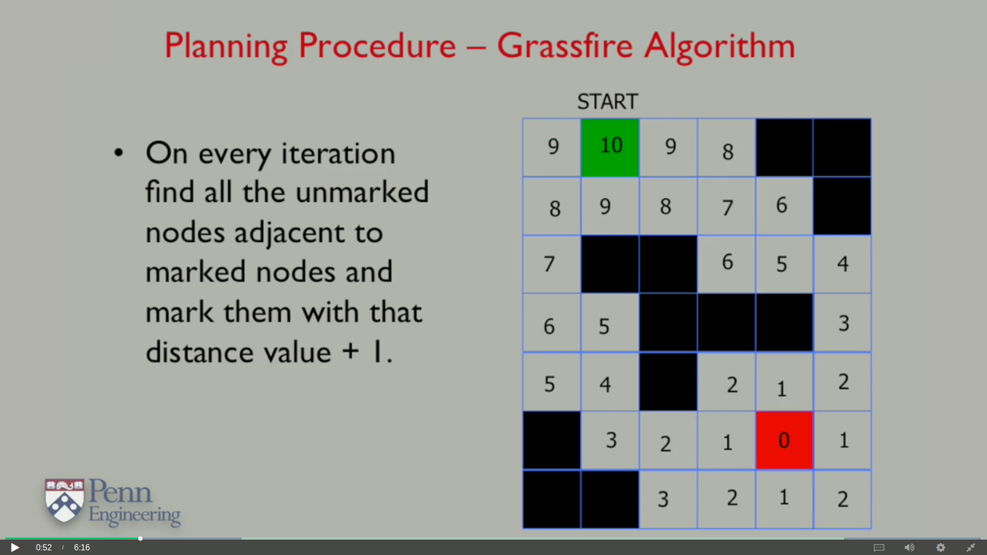
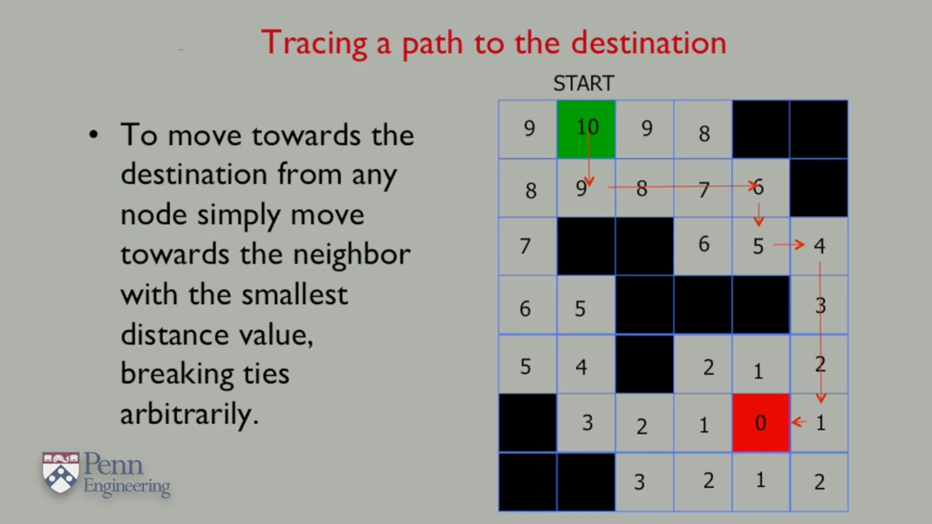
The destination cell is marked as 0 and the adjacent cells are marked in the increasing number sequence till we reach the starting cell.These numbers indicate the minimum number of steps required to reach the destination cell from that current cell.
Computation Complexity increases linearly with number of cells. For 2D grid 100 X 100 it is 10^4 For 2D grid 1000 X 1000 it is 10^6
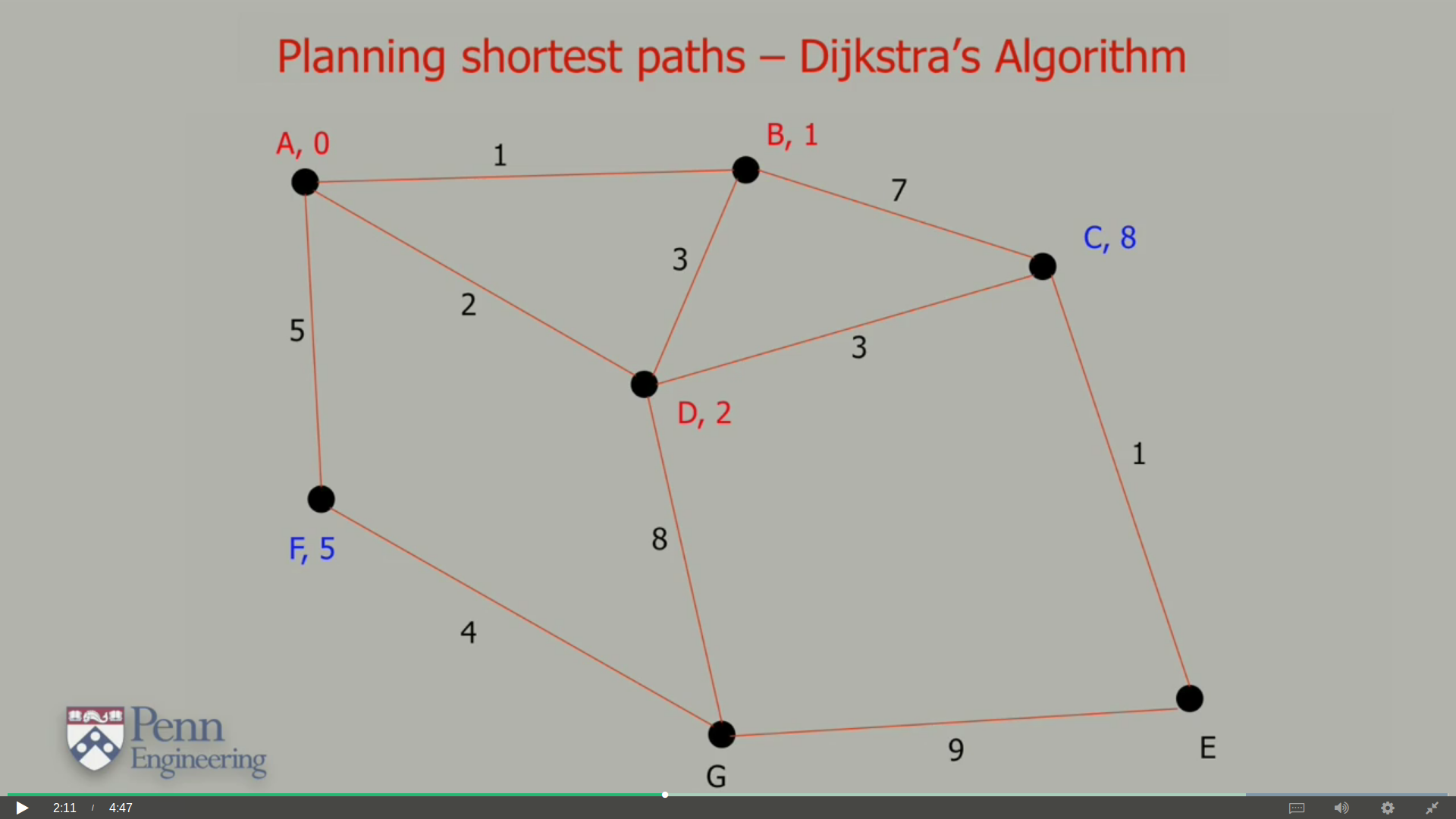
Start and Destination nodes along with many intermediate nodes like B,C,D are considered for path planning . Going along a path from one node to other carries a cost along with it . Our aim is to minimise this cost while going from Start to End .
Computation Complexity increses quadratically with the number of nodes.
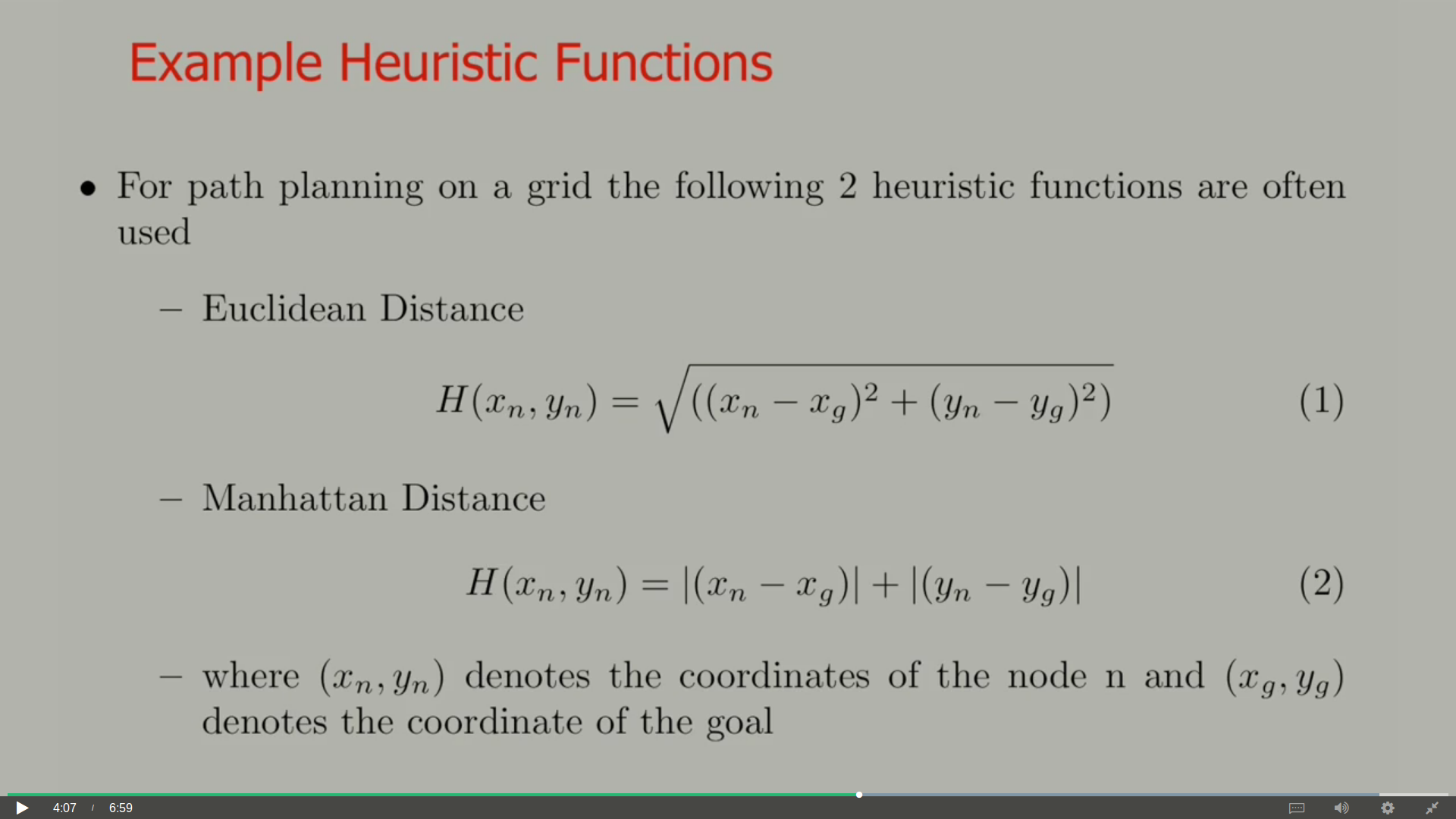
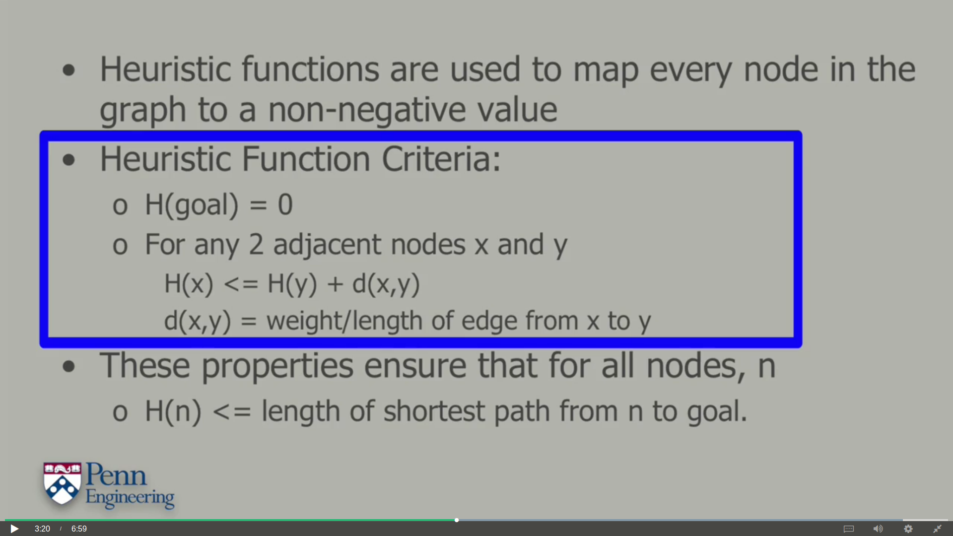
It introduces the idea of heuristic destination . It implies the concept that the minimum distance is encountered in the direction of destination . Although , sometimes we might be wrong due to some obstacle is encountered in between and we might need to head in the opposite direction .
Some common Heuristic Functions are Euclidean distance and Manhattan Distance. We proceed to neighboring node closest to the destination and then update the neighbors of the node .

It is the steerable space of the robot . This figure shows the tx, ty configurations that the robot cannot attain because of the obstacle. The dimensions and shape of the configuration space obstacle are obtained by considering both the obstacle and the shape of the robot. The configuration space obstacle is defined by what's known as the Minkowski sum of the obstacle and the robot shape. The configuration of the robot corresponds to a point in the configuration space. And the dark areas correspond to configurations that the robot cannot attain.

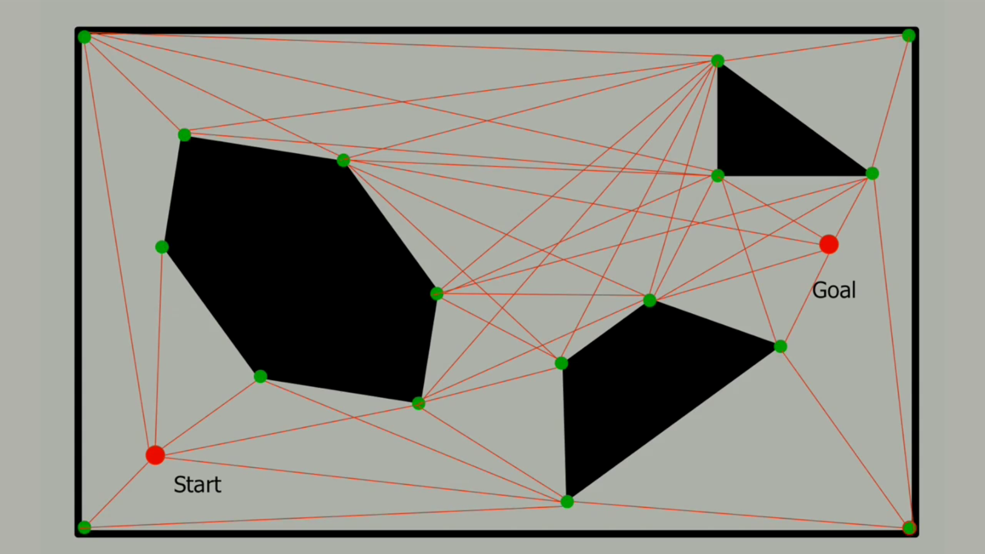

We draw an edge between any two vertices that can be connected by a straight line that lies entirely in free space. This visibility graph algorithm is actually complete.That is, it will find a path if one exists and report failure if no path can be constructed. This could happen if the start position or end position was entirely surrounded by an obstacle. Moreover, you can prove that this visibility algorithm are actually construct the shortest possible path between the two points.
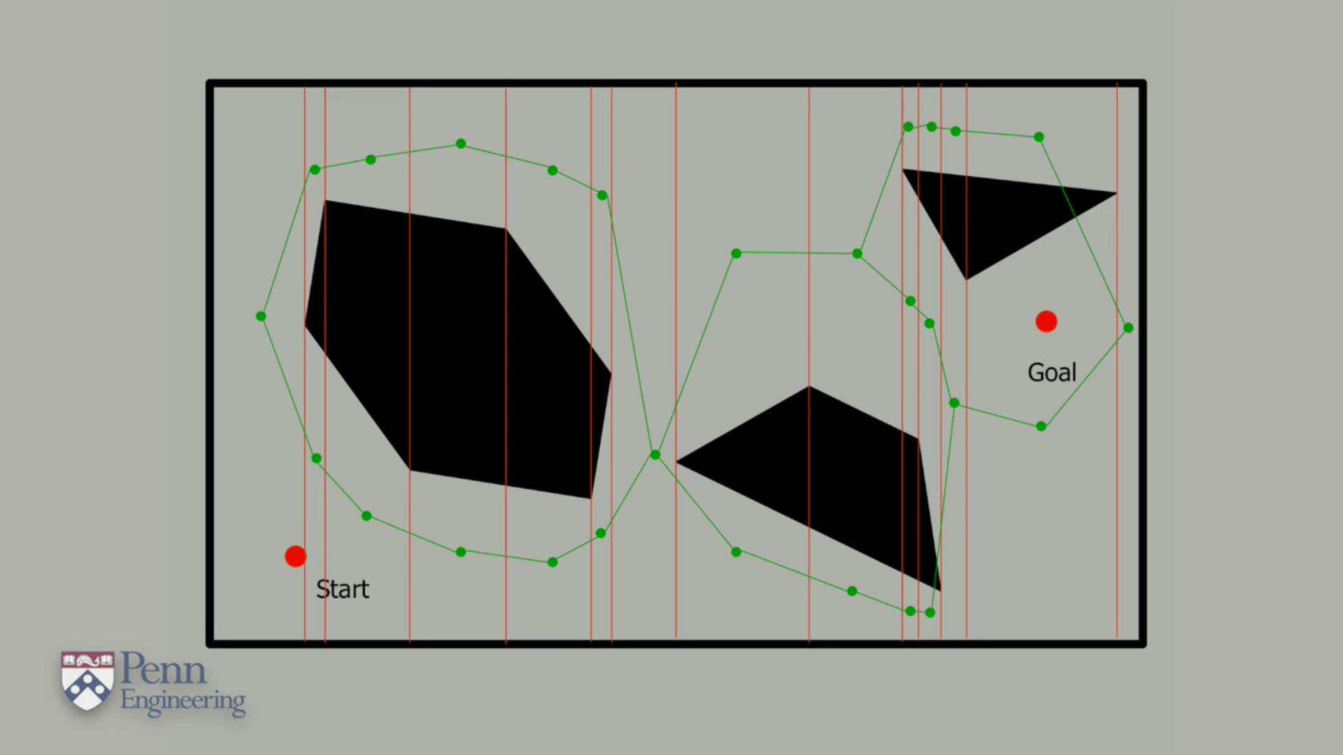
The nice thing about this is that these shapes are convex, which means that the robot can safely move in a straight line between any two points in each of the cells. As we said earlier we can form a graph where the nodes are these trapezoidal regions of free space and the edges indicate which of these regions are adjacent to each other. Path planning is then carried out by finding out which cell contains the start location and which the goal.And then planning a path through the graph between these two nodes.
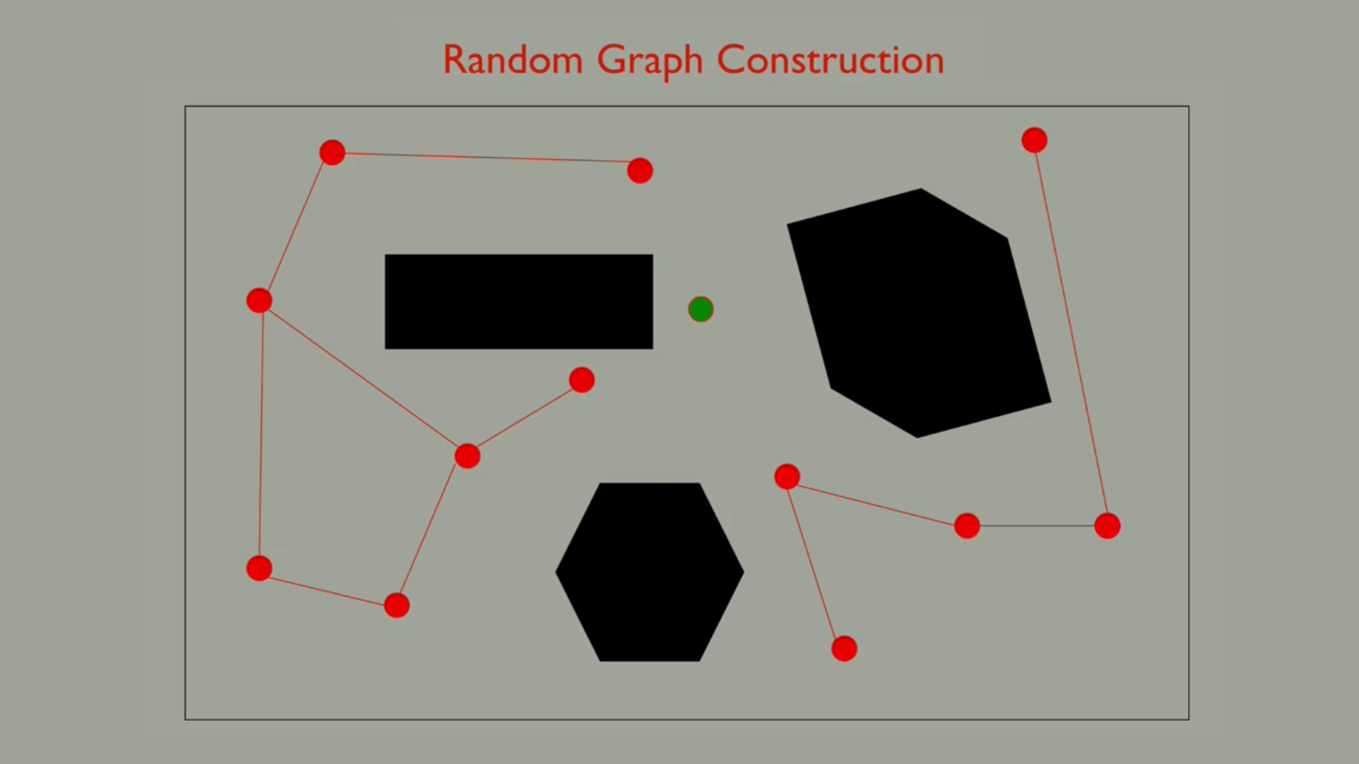
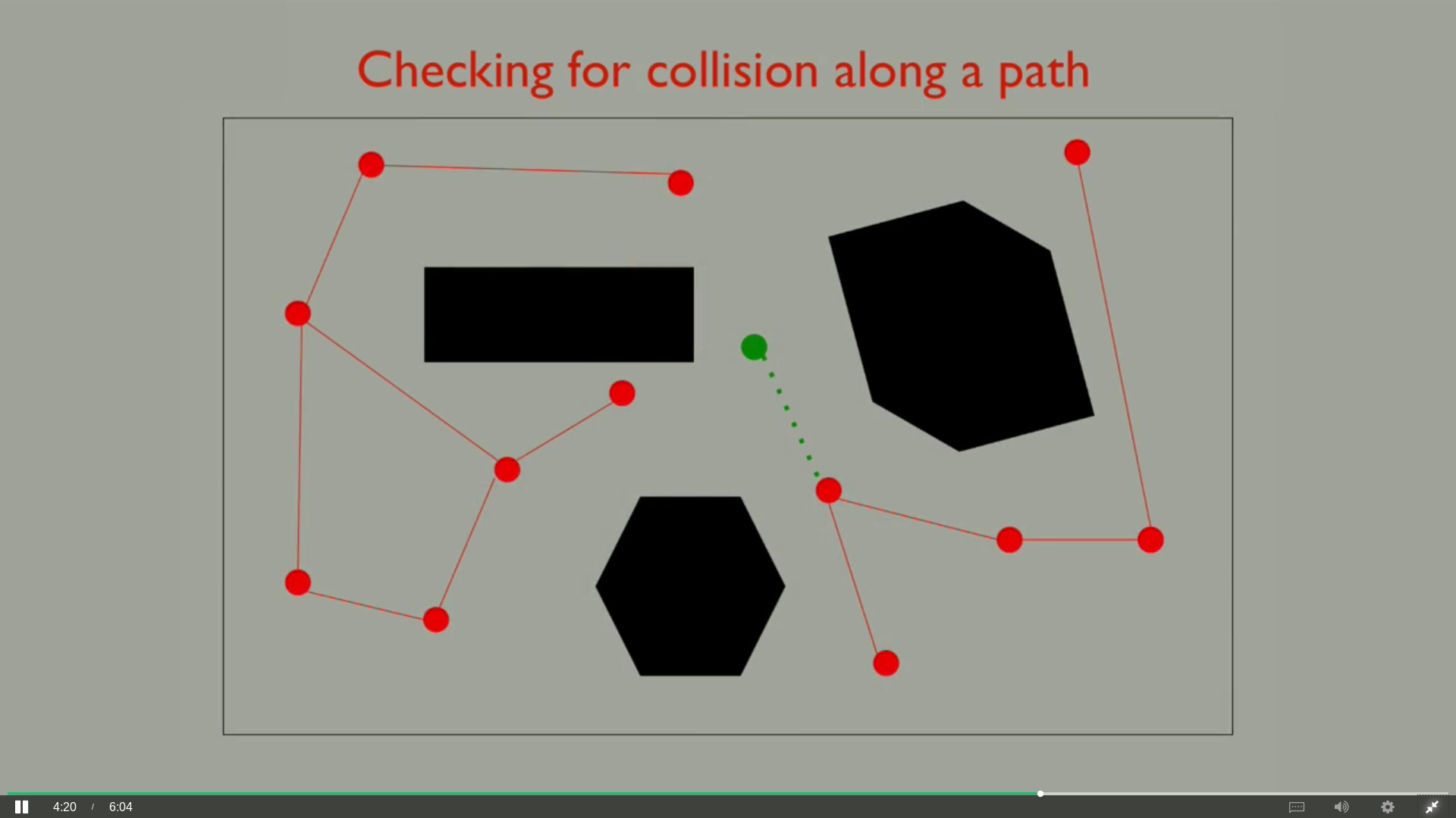
An alternative idea for dealing with these situations is to choose the points in the configuration space randomly instead of uniformly. In the hope that we will choose a set of configurations that capture the underlying structure of the free space. This illustrates the basic idea on a two dimensional configuration space. On every iteration, the system chooses a configuration in the configuration space at random, and tests whether it is in free space using the collision check function.
If it is in free space, it then tries to see if it can forge routes between this new configuration and the closest existing samples in the graph. Every path that it creates is recorded as a new edge in the graph that the system is building.
In this figure, the solid green lines correspond to new links that are added, while the dashed green line represents a connection that failed due to collision with the obstacle.
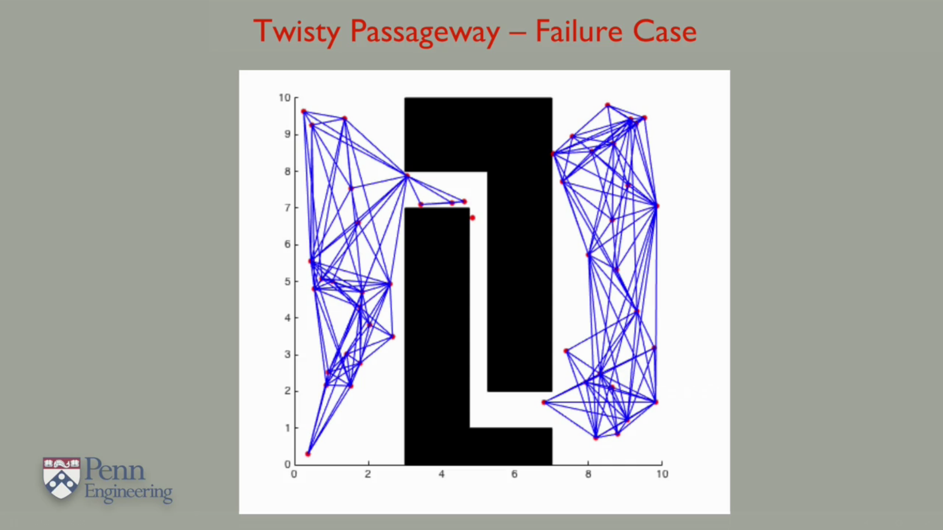
Problem with Probablistic Road Map A complete path planning algorithm would find a path if one existed, and report failure if it didn't. With the PRM procedure, it is possible to have a situation where the algorithm would fail to find a path even when one exists. If the sampling procedure fails to generate an appropriate set of samples. For example, the situation shown in this figure where there is a path but it involves finding a route through this small passageway. In order to find this route, a sampling algorithm would have to randomly generate samples in that narrow area.
The RRT procedure proceeds by constructing a special kind of graph called a tree, where every node is connected to a single parent and the tree is rooted at a given starting location. The following animation shows how the algorithm evolves to construct a tree in a two-dimensional configuration space containing obstacles.
On every iteration, the system generates a random point in the configurations base and checks if there's a free space. It then searches for the closest point in the existing tree and tries to generate a new node in the tree by moving in a straight line between the current vertex of the tree and new random vertex.
If the procedure does not succeed in this process of stepping towards a random node, it's simply abandons a point and moves on to the next iteration where it will generate a new random node.
In order to construct a path between the stark configuration and an end configuration, we actually construct two trees. One rooted at the start location and one at the goal. The procedure then tries to grow both trees until they meet. On every iteration of the algorithm, the system generates a random sample and tries to grow the current tree towards that random sample. If it succeeds in adding a new node to the tree, it tries to connect that new node to the other tree to form a bridge.
Note that if you succeed in finding such a bridge, you can claim success since it means that you have now forged a path between the two trees. On every route of this procedure, it swaps the two trees. That way, both trees are growing towards each other at the same rate.
In practice, the RRT Method is very effective at forging paths in high-dimensional configuration spaces. Another important feature of the RRT approach is it can be used on systems that have dynamic constraints, which limit how they can move.
References http://paper.ijcsns.org/07_book/201610/20161004.pdf
- Home
- Setup Your Computer
- Toolchain Installation
- Rotation Matrix and Quaternion
- PX4
- How to use aruco_ros
- Simulation using offboard control
- Resources
- Path Planning Algorithms