Refactor building of hydro profiles from EIA BA-level shapes to include EIA 923 information

[danielolsen]

🚀

• Is your feature request essential for your project?

Describe the workflow you want to enable

Currently, when building hydro profiles for the HIFLD grid model using prereise.gather.griddata.hifld.data_process.profiles.build_hydro, we use the balancing-authority-aggregated generation shape (after filtering and imputing) to populate the time-series profile for each hydro plant. There is additional information we could incorporate into these profiles however: information from EIA Form 923 which provides monthly net generation on a plant-level resolution.

Context

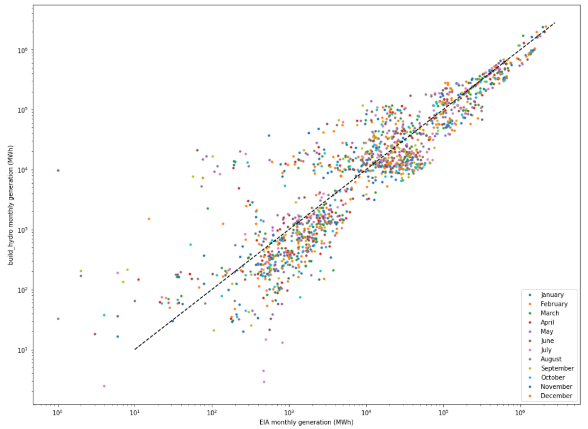
Looking at the existing time-series outputs of build_hydro and comparing to values from EIA 923, we see pretty significant differences, mostly for the smaller generators+month combinations but some significant differences exist for the larger ones as well.

For 2020 (the most recent year of full final data), the r-squared is 0.895, which seems pretty good! Raw MAPE is about 1200% for the 1,389 matching plants (seems pretty bad), although when we weight this by the generation for each (plant + month) combination, the weighted MAPE is about 40%: much better, but still not great. Part of this could be that there is a large chunk of data missing for CISO in this year, so CISO plants use an averaged profiles of all the other BAs. The following plots all show the same information, with different axis scales:

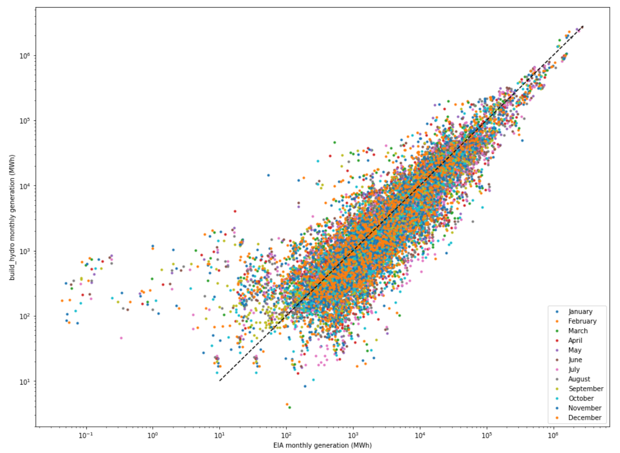
For 2021 (final data not yet available), there are only 135 matching plants (only those reporting monthly). The raw MAPE is worse than 2020, nearly 1600%, but the weighted MAPE is better, about 34%, and the r-squared is 0.897.

Code to reproduce (with the hifld branch of PreREISE checked out):

import matplotlib.pyplot as plt
import numpy as np
import pandas as pd
from scipy.stats import linregress
from prereise.gather.griddata.hifld.data_process.profiles import build_hydro
from prereise.gather.griddata.hifld.orchestration import create_grid

# Define a function to report results for an arbitrary year
def compare_monthly_generation(hydro_plants, eia_923_df, year):
    def plot_by_month(parsed_eia_923_df, monthly_hydro):
        fig = plt.figure(figsize=(16,12))
        ax = fig.add_subplot()
        for month_num, month_name in months.items():
            plt.plot(
                parsed_eia_923_df.loc[month_num, common_plant_codes],
                monthly_hydro.loc[month_num, common_plant_codes],
                '.',
                label=month_name,
            )
        plt.plot([1e1, 2.8e6], [1e1, 2.8e6], 'k--')
        plt.legend()
        plt.xlabel("EIA monthly generation (MWh)")
        plt.ylabel("build_hydro monthly generation (MWh)")
        return ax

    # Build time-series hydro profiles from Balancing authority shapes
    hourly_hydro = build_hydro(
        hydro_plants.set_index("Plant Code"),
        eia_api_key=eia_api_key,
        year=year,
    )
    # Parse hourly to monthly
    monthly_hydro = (
        hourly_hydro.groupby(hourly_hydro.index.month).sum()
        * hydro_plants.set_index("Plant Code")["Pmax"]
    )
    # Interpret raw EIA 923 data to (month x plant_code) data frame
    parsed_eia_923_df = (
        eia_923_df
        .loc[
            (eia_923_df["Reported\nPrime Mover"] == 'HY')
            & (eia_923_df["Plant Id"] != 99999),
            ["Plant Id"] + list(eia_923_cols_of_interest)
        ]
        .replace(".", float("nan"))
        .groupby("Plant Id").sum()
        .astype(float)
        .rename(eia_923_cols_of_interest, axis=1)
        .T
    )
    # Identify which Plant Codes match across data sets
    common_plant_codes = set(parsed_eia_923_df.columns) & set(monthly_hydro.columns)
    print(len(common_plant_codes), "matching plant codes")
    # Make plots
    ax = plot_by_month(parsed_eia_923_df, monthly_hydro)
    plt.show()
    ax = plot_by_month(parsed_eia_923_df, monthly_hydro)
    ax.set_xlim(0, 5e5)
    ax.set_ylim(0, 5e5)
    plt.show()
    ax = plot_by_month(parsed_eia_923_df, monthly_hydro)
    ax.set_xscale("log")
    ax.set_yscale("log")
    plt.show()
    # Calculate statistics
    raveled_923 = np.ravel(parsed_eia_923_df[common_plant_codes])
    raveled_hydro = np.ravel(monthly_hydro[common_plant_codes])
    total_length = raveled_923.shape[0]
    ape = np.zeros(total_length)
    for i in range(total_length):
        if raveled_923[i] in {float("nan"), ".", 0}:
            ape[i] = float("nan")
        else:
            ape[i] = abs((raveled_hydro[i] - raveled_923[i]) / raveled_923[i])
    good_data_mask = ~np.isnan(ape)
    mape = np.mean(ape[good_data_mask])
    print(f"{mape=}")
    weighted_mape = (
        np.sum((ape * np.ravel(parsed_eia_923_df[common_plant_codes]))[good_data_mask])
        / np.sum(np.ravel(parsed_eia_923_df[common_plant_codes])[good_data_mask])
    )
    print(f"{weighted_mape=}")
    slope, intercept, rvalue, pvalue, stderr = linregress(
        raveled_923[good_data_mask], raveled_hydro[good_data_mask]
    )
    print("r-squared", rvalue**2)

# Constants
eia_api_key = YOUR_EIA_API_KEY_HERE
months = {
    1: "January",
    2: "February",
    3: "March",
    4: "April",
    5: "May",
    6: "June",
    7: "July",
    8: "August",
    9: "September",
    10: "October",
    11: "November",
    12: "December",
}
eia_923_cols_of_interest = {f"Netgen\n{v}": k for k, v in months.items()}

# Build the HIFLD grid without dropping columns that are irrelevant to PowerSimData
# This step can take a while, depending on what you have cached
# Go grab a cup of coffee while you wait
full_tables = create_grid()
# Read 2020 data, generate 2020 hydro, compare
eia_923_2020 = pd.read_excel(
    PATH_TO_YOUR_LOCAL_EIA_FORM_923_2020_FILE,
    header=5
)
compare_monthly_generation(full_tables["plant"].query("type == 'hydro'"), eia_923_2020, 2020)
# Read 2021 data, generate 2021 hydro, compare
eia_923_2021 = pd.read_excel(
    PATH_TO_YOUR_LOCAL_EIA_FORM_923_2021_FILE,
    header=5
)
compare_monthly_generation(full_tables["plant"].query("type == 'hydro'"), eia_923_2021, 2021)

Describe your proposed implementation, if applicable

build_hydro is refactored to be able to (potentially toggled by a feature flag) scale the hourly BA-level shapes to better represent the monthly energy totals from EIA 923. I believe this information can be retrieved from the EIA's API using the same API key as we use to grab the BA-level hydro generation, or alternatively could be retrieved from an alternate source (see #246). Using a naive scaling factor based on (EIA 923 monthly energy / build_hydro monthly energy) could be problematic since it could result in values which are greater than 1 during some hours. If we use this approach, we'll need to be sure to clip these values to be no larger than 1.

EIA Form 923 also seems to sometimes contain distinct entries for conventional hydro ("Reported Prime Mover" == "HY") vs. pumped storage hydro ("Reported Prime Mover" == "PS") within the same Plant Code entry, and reports the 'fuel consumed' for pumping. We may be able to use this information to identify which plants are pumped storage (and whose profiles can therefore go negative) vs. which plants are conventional hydro only (and should have their profiles clipped to a minimum of 0).

[victoriahunt]

Proposed implementation plan, part 1: refactor build_hydro and add a feature flag (toggle). Goal of the feature is to better represent the monthly energy totals from EIA 923. "Better represent" will be assessed on the basis of R^2 and MAPE, comparing against prior metrics generated by Daniel O. and reported in the issue. The code provided in the issue can be used to directly assess these metrics. Actual values for 2020 will be retrieved with the same API key as we use to grab the BA-level hydro generation. Actual values will also be used to create scaling factors which will be applied to our profiles.

Plan part 2: Identify pumped hydro vs. conventional hydro and clip profile of conventional hydro with minimum value of 0. Assess against R^2 and MAPE to see if this is an improvement. If so, implement this additional improvement.