Convolutional networks, also known as convolutional neural networks or CNNs, are a specialized kind of neural network for processing data that has a known, grid-like structure.
CNNs are mostly used to solve computer vision problems i.e. image processing. They can identify faces, individuals, street signs, platypuses, and many other aspects of visual data. CNNs overlap with text analysis via optical character recognition, but they are also useful when analyzing words as discrete textual units. They are also good at analyzing sound. From image classification to object detection, CNNs are being used to diagnose cancer patients and detect fraud in systems, as well as to construct well-thought-out self-driving vehicles that will revolutionize the future. The best convolutional neural networks today reach or exceed human-level performance, a feat considered impossible by most experts in computer vision only a couple of decades back.
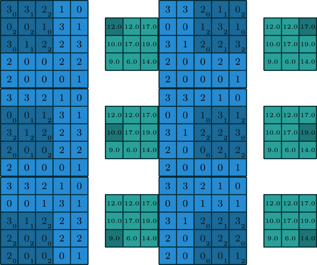
CNNs use filters called convolutional kernels to transform their input through multiple layers and return a feature map of the original input as a result. They use a mathematical operation known as a convolution in place of general matrix multiplication in at least one of their layers. Convolution, or more precisely, discrete convolution, is defined for a 2D image as the scalar product of a weight matrix, called the kernel, with every neighborhood in the input. In other words, the kernel "slides" over the 2D input data, performing an elementwise multiplication with the part of the input it is currently on, and then summing up the results into a single output pixel.
After performing a convolution over the entire image, each output pixel is run through a nonlinear activation function, such as the rectified linear activation (ReLU) function. This stage is sometimes called the detector stage. Finally, a CNN uses pooling layers to reduce the resolution of the network from the previous input layer, which gives us fewer parameters in lower layers.
This is the first step in extracting features from an image. The objective is to maintain the relationship between nearby pixels by learning the features over small sections of the image. If we have a grayscale image, it consists of an array, x pixels wide and y pixels high, with each entry having a value that indicates whether it’s black or white or somewhere in between (assuming an 8-bit image, each value can vary from 0 to 255). We use a filter, or convolutional kernel, which is another matrix, most likely smaller than the image, which we will drag across our image. To produce our output, we take the smaller filter and pass it over the original input, like a magnifying glass over a piece of paper. All we do is multiply each element in the matrix by its corresponding member in the other matrix and sum the result.
We repeat this process for the entire image, giving us the final result, also known as feature/activation map. Our goal is to learn the best possible convolutional kernel for an image.
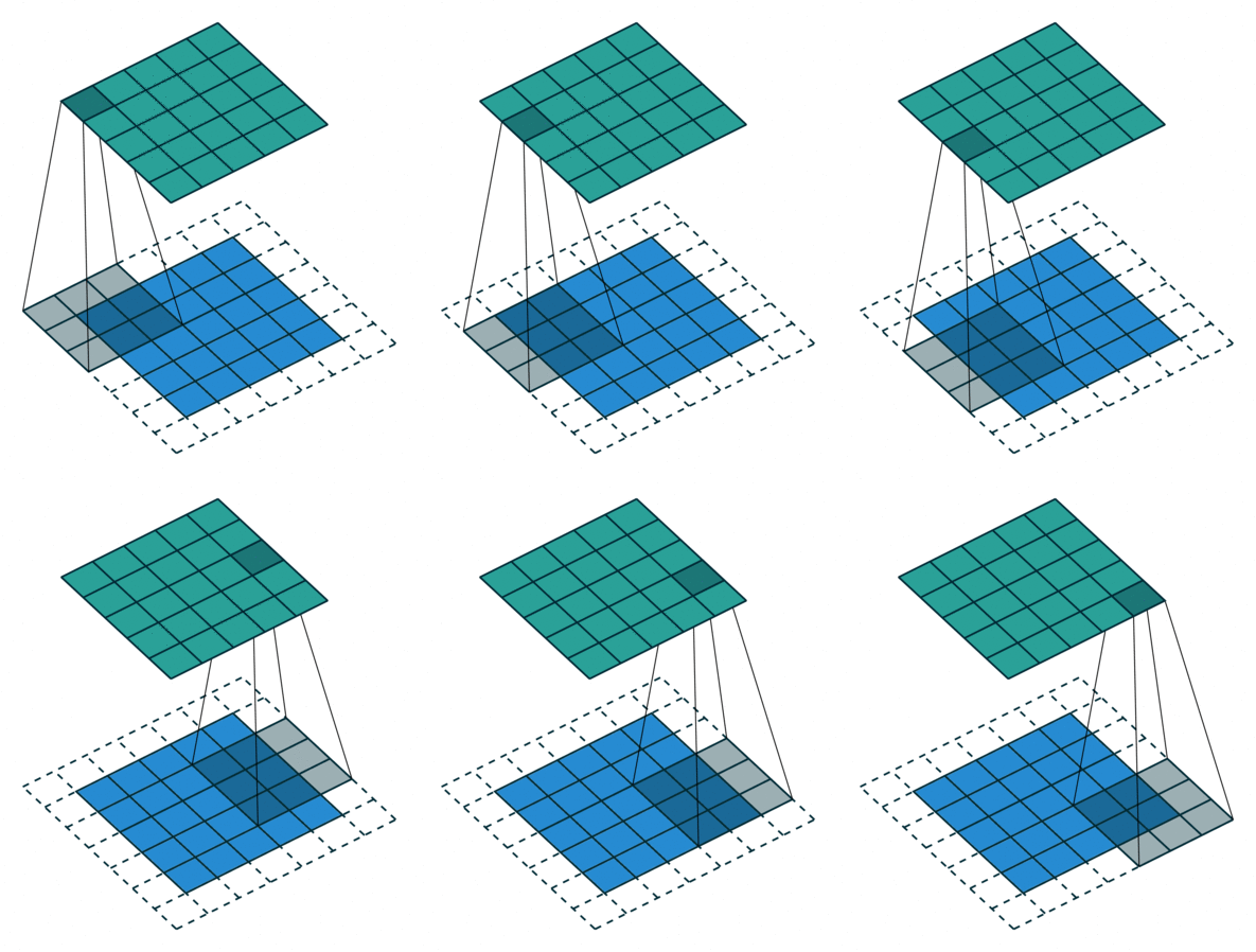
- Padding: If you notice the above animation, the feature map is 3x3 whereas the original image is 5x5. This is because the pixels on the edges are trimmed off.
The pixels on the edge are never at the center of the kernel, because there is nothing for the kernel to extend to beyond the edge.
This isn’t ideal, as often we’d like the size of the output to equal the input. Padding does something pretty clever to solve this:
pad the edges with extra, "fake" pixels (usually of value 0, hence the oft-used term "zero padding").
This way, the kernel when sliding can allow the original edge pixels to be at its center, while extending into the fake pixels beyond the edge, producing an output the same size as the input.
- Stride: Indicates how many steps across the input we move when we adjust the filter to a new position. The above example has a stride of 1. If it had a stride of 2, the feature map would have half its size.
Whereas in the 1 channel case, where the term filter and kernel are interchangeable, in the general case, they’re actually pretty different. Each filter actually happens to be a collection of kernels, with there being one kernel for every single input channel to the layer, and each kernel being unique. Each of the kernels of the filter "slides" over their respective input channels, producing a processed version of each. Some kernels may have stronger weights than others, to give more emphasis to certain input channels than others (e.g. a filter may have a red kernel channel with stronger weights than others, and hence, respond more to differences in the red channel features than the others). Each of the per-channel processed versions are then summed together to form one channel. The kernels of a filter each produce one version of each channel, and the filter as a whole produces one overall output channel. Finally, then there's the optional bias term. The way the bias term works here is that each output filter has one bias term. The bias gets added to the output channel so far to produce the final output channel.
A pooling function replaces the output of the net at a certain location with a summary statistic of the nearby outputs. Pooling layers commonly reduce the input's height and width by half. Pooling layers aim to reduce the number of parameters in the network by keeping the most relevant features. A common pooling function is the max pooling operation that takes the maximum element from a rectangular neighborhood. For example, a (2x2) pooling layer would choose the maximum element from a (2x2) subsection of the feature map. An alternative to maximum pooling is average pooling, which takes the arithmetic mean of a rectangular neighborhood. This means that if the input image were 32 pixels wide by 32 pixels tall, the output image would be smaller in width and height (e.g., 16 pixels wide by 16 pixels tall).
Where does this end? After the input image has been reduced to a small set of features, we expect to be able to output some probabilities from the network that we can feed to our negative log likelihood. For this reason, the feature map is flattened to a 1D vector and passed to a fully-connected layer that outputs probabilities.
There are certain advantages offered by convolutional layers when working with image data:
- Fewer parameters: A small set of parameters (the kernel) is used to calculate outputs of the entire image, so the model has much fewer parameters compared to a fully connected layer.
- Sparsity of connections: In each layer, each output element only depends on a small number of input elements, which makes the forward and backward passes more efficient.
- Parameter sharing and spatial invariance: The features learned by a kernel in one part of the image can be used to detect similar pattern in a different part of another image.
- LeNet18
- One of the earliest successful architectures of CNNs
- Developed by Yann Lecun
- Originally used to read digits in images
- AlexNet19
- Helped popularize CNNs in computer vision
- Developed by Alex Krizhevsky, Ilya Sutskever, and Geoff Hinton
- Won the ILSVRC 2012
- ZF Net20
- Won the ILSVRC 2013
- Developed by Matthew Zeiler and Rob Fergus
- Introduced the visualization concept of the Deconvolutional Network
- GoogLeNet21
- Won the ILSVRC 2014
- Developed by Christian Szegedy and his team at Google
- Codenamed “Inception,” one variation has 22 layers
- VGGNet22
- Runner-Up in the ILSVRC 2014
- Developed by Karen Simonyan and Andrew Zisserman
- Showed that depth of network was a critical factor in good performance
- ResNet23
- Trained on very deep networks (up to 1,200 layers)
- Won first in the ILSVRC 2015 classification task
- Goodfellow, I., Bengio, Y., & Courville, A. (2016). Deep Learning. MIT Press. http://www.deeplearningbook.org
- Saleh, H. (2020). The Deep Learning with PyTorch Workshop. Packt Publishing Ltd.
- Shafkat, I. (2018, June 2). Intuitively Understanding Convolutions for Deep Learning. Medium. https://towardsdatascience.com/intuitively-understanding-convolutions-for-deep-learning-1f6f42faee1

