01_Pose_Graph.md

References

Pose Graph Papers

1. 2013: Information fusion in navigation systems via factor graph based incremental smoothing
2. 2018: Laser-visual-inertial Odometry and Mapping with High Robustness and Low Drift
3. 2020: LIO-SAM: Tightly-coupled Lidar Inertial Odometry via Smoothing and Mapping
   • Proposing LiDAR odometry factor
   • The obtained lidar odometry solution is then used to estimate the bias of the IMU in the factor graph.
   • Loop Closure factor
   • Lidar/IMU/GPS

4. 2021: LVI-SAM: Tightly-coupled Lidar-Visual-Inertial Odometry via Smoothing and Mapping
   • Lidar/IMU/GPS/Vision
     

Pose Graph

source: hal

Markov Chain	Factor Graph

• The maximum a posteriori (MAP) estimate is given by x= argmax p(x|z).
• x: is all the states (that we want to get)
• z: all the sensor measurmnets

   Σ can come from VAE

iSAM2

Name	Equation
A factor graph is a bipartite graph
Factor nodes
Variable nodes
Edges
A factor graph G defines the factorization of a function f (Θ) as: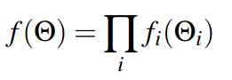
(where Θi is the set of variables θ j adjacent to the factor fi, and independence relationships are encoded by the edges eij)
Goal is to find the variable assignment Θ∗ that maximizes f:
Assuming Gaussian measurement models: (h: measurment fun., z: measurmnet)
Corresponds to the nonlinear least-squares criterion
Squared Mahalanobis distance with covariance matrix Σ
The Mahalanobis distance is a measure of the distance between a point P and a distribution D. It is a multi-dimensional generalization of the idea of measuring how many standard deviations away P is from the mean of D
In practice one typically considers a linearized version of problem (min)

Bayes theorem

Probability

Let Y be N(μ,σ2), the normal distrubution with parameters μ and σ2.

• The density function of Y is
  

• Probability for a distribution is associated with the area under the curve for a particular range of values
  

• The n-th central moment of Y is
  

• If the function is a probability distribution, then the first moment is the expected value, the second central moment is the variance, the third standardized moment is the skewness
  

Probability vs. Likelihood

• Probability is the percentage that a success occur.
• Likelihood is the probability (conditional probability) of an event (a set of success) occur by knowing the probability of a success occur.

  

Marginalisation

• Marginalisation is a method that requires summing over the possible values of one variable to determine the marginal contribution of another.
• Marginalization is a process of summing a variable X which has a joint distribution with other variables like Y, Z, and so on. Considering 3 random variables, we can mathematically express it as
  

Maximization

Expected Value- Variance -Covariance NUMPY

Expected Value

In probability, the average value of some random variable X is called the expected value or the expectation. mean, average, and expected value are used interchangeably

• E[X] = sum(x1 * p1, x2 * p2, x3 * p3, ..., xn * pn)
• mu = sum(x1, x2, x3, ..., xn) . 1/n
• mu = sum(x . P(x))

Variance

In probability, the variance of some random variable X is a measure of how much values in the distribution vary on average with respect to the mean

• Var[X] = E[(X - E[X])^2]
• Var[X] = sum (p(x1) . (x1 - E[X])^2, p(x2) . (x2 - E[X])^2, ..., p(x1) . (xn - E[X])^2)
• sigma^2 = sum from 1 to n ( (xi - mu)^2 ) . 1 / (n - 1) (minus 1 to correct for a bias)

Covariance

• cov(X, Y) = E[(X - E[X]) . (Y - E[Y])]
• cov(X, Y) = sum (x - E[X]) * (y - E[Y]) * 1/n
• cov(X, Y) = sum (x - E[X]) * (y - E[Y]) * 1/(n - 1)

Maximum a posteriori estimation

Sources:

1
2.Equivariant Neural Network for Factor Graphs