RBF (Network) has some relationhsip with SVM (kernel), kNN, k-Means, Neural Network
In multilayer perceptron, the input is encoded by the simultaneous activation of many hidden units. This is called a Distributed Representation.
But in RBF, for a given input, only one or a few units are active. This is called a Local Representation.
Receptive Field: The part of the input space where a unit has nonzero response. (Like in SVM, only Support Vector (some of the decisive input data) will participate in the decision.)
smaller
$M$ and larger$\lambda$
Choosing Prototype by k-Means Clustering
using unsupervised learning (k-Means) to assist feature transform (like autoencoder)
Gaussian SVM: find
The Gaussian kernel is also called RBF kernel
- Radial: only depends on distance between
$x$ and 'center'$x_n$ - Basis Function: to be 'combined'
let
Linear aggregation of selected radial hypothesis
kernel: similarity via inner product in
$\mathcal{Z}$ -spaceRBF: similarity via
$\mathcal{X}$ -space distance (often monotonically non-increasing to distance)
Linear aggregation of radial hypotheses
It's a simple (old-fashioned) model
The difference between normal neural network
| - | Normal Neural Network | RBF Network |
|---|---|---|
| hidden layer | inner product + activation function | distance of centers + Gaussian |
| output layer | linear aggregation | linear aggregation |
| layer number | may have multiple layers | normally no more than one layer of Gaussian units |
RBF Network is historically a type of neural netowrk
The Learning Variables:
-
centers
$\mu_m$ - (signed) votes
$\beta_m$ (the linear aggregation weight)
When
Full RBF Network has some relation with kNN
Formula Corresponding
- RBF vs. Gaussian
- Output activation function vs. Sign function (for binary classification)
-
$M$ vs. number of support vector -
$\mu_m$ vs. SVM support vector$x_m$ -
$\beta_m$ vs.$\alpha_my_m$ from SVM Dual
RBF Network: distance similarity-to-centers as feature transform
Parameters
-
$M$ : prototypes (centroid) - RBF: such as
$\gamma$ of Gaussian
Non-regularized Full RBF Network
called exact interpolation for function approximation. this is bad in machine learning => overfitting
Regularized Full RBF Network
... (around 15 mins in Hsuan-Tien Lin Machine Learning Techniques RBF Network Learning)
Basically the Exercises 3 and 4 in Introduction to Machine Learning 3rd Ch12.11
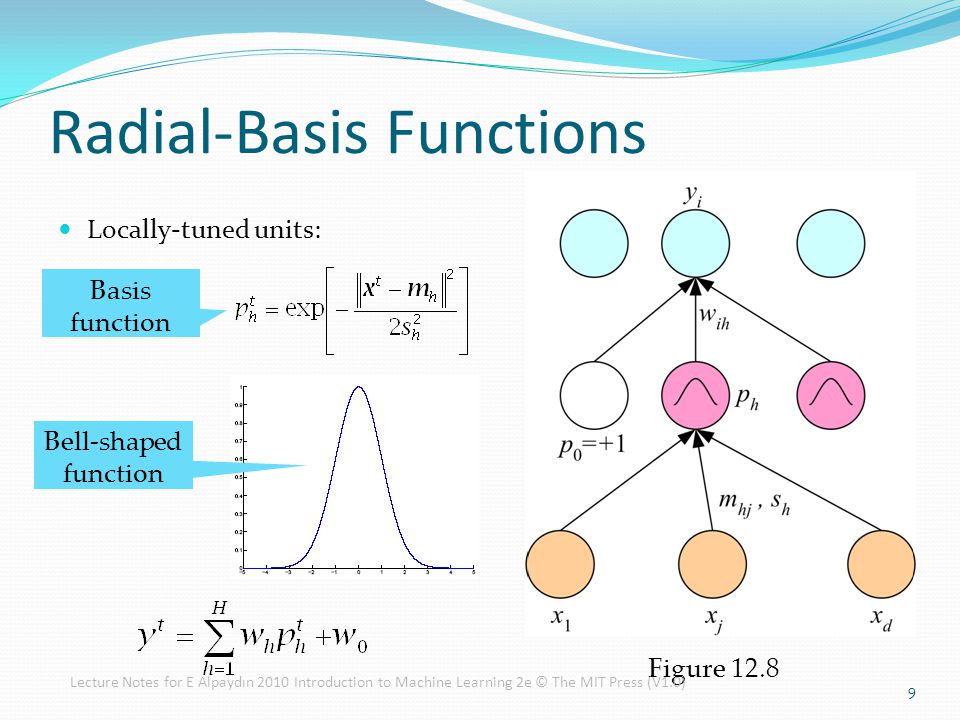
Figure 12.8
The RBF network where
Equation 12.20 - the softmax
$$ y_{i}^{t}=\frac{\exp \left[\sum_{h} w_{i h} p_{h}^{t}+w_{i 0}\right]}{\sum_{k} \exp \left[\sum_{h} w_{k h} p_{h}^{t}+w_{k 0}\right]} $$ Equation 12.21 - the cross-entropy error
$$ E\left(\left{\mathbf{m}{h}, s{h}, w_{i h}\right}{i, h} | X\right)=-\sum{t} \sum_{i} r_{i}^{t} \log y_{i}^{t} $$
Because of the use of cross-entropy and softmax, the update equations will be the same with equations 12.17, 12.18, and 12.19 (see equation 10.33 for a similar derivation).
Equation 12.17 - the update rule for the second layer weights
Equation 12.18, 12.19 - the update equations for the centers and spreads by backpropagation (chain rule)
Equation 10.33
Equation 12.22
$$ y^{t}=\underbrace{\sum_{h=1}^{H} w_{h} p_{h}^{t}}{\textit{exceptions}}+\underbrace{\mathbf{v}^{T} \mathbf{x}^{t}+v{0}}_{rule} $$
There are two sets of parameters:
$\mathbf{v}$ ,$v_0$ of the default model and$w_h$ ,$\mathbf{m}_h$ ,$s_h$ of the exceptions. Using gradient-descent and starting from random values, we can update both iteratively. We update$\mathbf{v}$ ,$v_0$ as if we are training a linear model and$w_h$ ,$\mathbf{m}_h$ ,$s_h$ as if we are training a RBF network.Another possibility is to separate their training: First, we train the linear default model and then once it converges, we freeze its weights and calculate the residuals, that is, differences not explained by the default. We train the RBF on these residuals, so that the RBF learns the exceptions, that is, instances not covered by the default “rule.”
- Intorduction to Machine Learning 3rd Ch12 Local Models
- Ch12.3 Radial Basis Functions
- Ch12.11 Exercises
- 3
- 4
- Radial basis function - 徑向基函數
- Radial basis function kernel
- Radial basis function network
- Radial basis function interpolation
- Hsuan-Tien Lin Machine Learning Techniques (機器學習技法) - Radial Basis Function Network
- CS 156 Lecture 16 - Radial Basis Functions

