Table of Contents
Probability
ML Concepts
ML Data Processing
- How do you handle data imbalance issues?
- How to deal with missing values? Mention three ways to handle missing or corrupted data in a dataset?
- You are given a data set with missing values that spread along 1 standard deviation from the median. What percentage of data would remain unaffected?
- How to deal with outliers? What are the data preprocessing techniques to handle outliers? Mention 3 ways that you prefer, with proper explanation.
- What is difference between Normalization, Standardization, Regularization?
- What is instance normalisation?
- Explain the bias-variance tradeoff.
- While analyzing your model’s performance, you noticed that your model has low bias and high variance. What measures will you use to prevent it (describe two of your preferred measures)?
- What is the difference between overfitting and underfitting?
- Explain regularization. When is 'Ridge regression' favorable over 'Lasso regression'?
- What is the degree of freedom for lasso?
- What do L1 and L2 regularization mean and when would you use L1 vs. L2? Can you use both?
- When there are highly correlated features in your dataset, how would the weights for L1 and L2 end up being?
- When is One Hot encoding favored over label encoding?
- What is the curse of dimensionality? Why do we need to reduce it? What is PCA, why is it helpful, and how does it work? What do eigenvalues and eigenvectors mean in PCA?
ML Training
- What is a Gradient?
- Explain Gradient descent and Stochastic gradient descent. Which one would you prefer?
- Mention one disadvantage of Stochastic Gradient Descent.
- Explain different types of Optimizers? How is 'Adam' optimizer different from 'RMSprop'? Explain how Momentum differs from RMS prop optimizer?
- What is the cross-entropy of loss? How does the loss curve for Cross entropy look? What does the “minus” in cross-entropy mean?
- Can you use MSE for evaluating your classification problem instead of Cross entropy?
- What is a hyperparameter? How to find the best hyperparameters?
Validation & Metrics
- Why is a validation set necessary?
- Can K-fold cross-validation be used on Time Series data? Explain with suitable reasons in support of your answer.
- Define precision, recall, and F1 and discuss the trade-off between them.
- Explain the ROC Curve and AUC. What is the purpose of a ROC curve?
NLP
- What techniques for NLP data augmentation do you know?
- Write term frequency–inverse document frequency function.
- 28 Probability Questions for ML Interviews
- Probability and Statistics for Software Engineering Problems
Explain the difference between Supervised and Unsupervised machine learning? What are the most common algorithms for supervised learning and unsupervised learning?
- In Supervised learning, the algorithm is trained on a labelled dataset, meaning the desired output is provided.
- In Unsupervised learning, the algorithm must find patterns and relationships in an unlabeled dataset.
Supervised Learning Algorithms
- Regression models (the output is continuous)
- Linear Regression
- Linear Support Vector Machines (SVMs)
- Naive Bayes
- Classification models (the output is discrete)
Unsupervised learning
- Principal Component Analysis (PCA)
- Clustering - Clustering is an unsupervised technique that involves the grouping, or clustering, of data points.
- K-Means Clustering
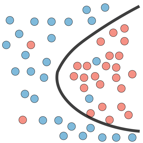
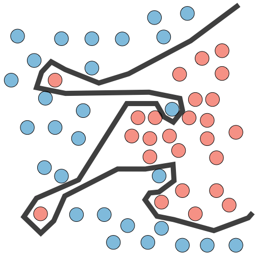
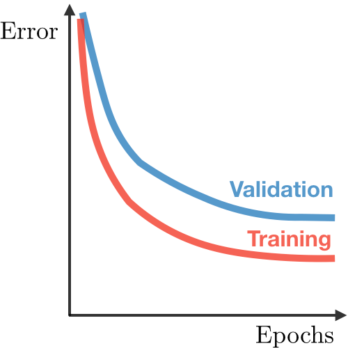
Overfitting occurs when a model learns to perform exceptionally well on the training data but fails to perform well on new, unseen data.
- Overfitting occurs when a model learns the training data too well, capturing even the noise or random fluctuations present in the data.
- Model is too complex and adapts to the training data’s peculiarities rather than learning the underlying pattern.
Underfitting occurs when a model is too simple and cannot capture the underlying pattern in the data, resulting in poor performance on both the training and test data.
- Model doesn’t have enough capacity or complexity to learn the true relationship between the input features and the target variable.
| Underfitting | Just right | Overfitting | |
|---|---|---|---|
| Symptoms | • High training error • Training error close to test error • High bias |
• Training error slightly lower than test error | • Very low training error • Training error much lower than test error • High variance |
| Regression illustration | 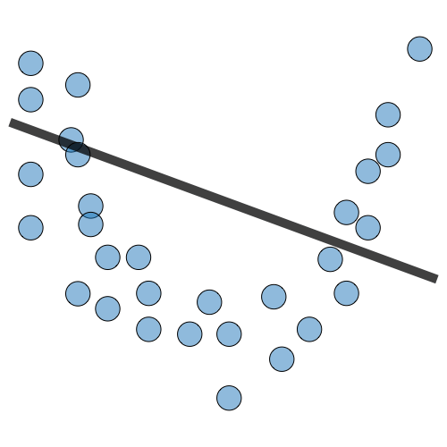 |
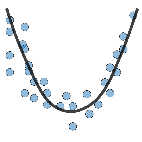 |
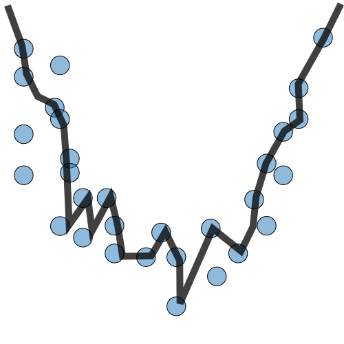 |
| Classification illustration | 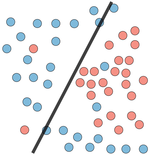 |
 |
 |
| Deep learning illustration | 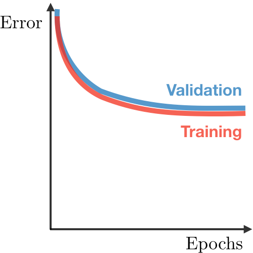 |
 |
 |
| Possible remedies | • Complexify model • Add more features • Train longer |
• Perform regularization • Get more data |
Both covariance and correlation measure the relationship and the dependency between two variables.
- Covariance indicates the direction of the linear relationship between variables
- Correlation measures both the strength and direction of the linear relationship between two variables.
Correlation is a function of the covariance.
Correlation:
High degree of covariance, it can negatively affect the performance of the linear regression model. Here are some ways that covariance affects linear regression models:
- Multicollinearity: High degree of covariance, can lead to multicollinearity. It can lead to inaccurate predictions and a lack of interpretability for the model.
- Overfitting: A high degree of covariance between the variables, can lead to overfitting because the model is trying to fit the noise rather than the underlying relationship.
Identify covariance in a linear regression model, consider the following strategies:
- Examine the correlation matrix
- Conduct a variance inflation factor (VIF) analysis: The VIF measures the extent to which the variance of a regression coefficient estimate is increased due to covariance with other variables in the model. A VIF greater than 1 indicates that there is some degree of covariance, and VIF values greater than 5 or 10 indicate that there are significant issues with multicollinearity.
Refer to Regularization Notes
Lasso will be unable to make model if there is multicollinearity.
When there are highly correlated features in your dataset, how would the weights for L1 and L2 end up being?
L2 regularization can keep the parameter values from going too extreme. While L1 regularization can help remove unimportant features.
| Lasso | Rasso | Elasitc Net |
|---|---|---|
| • Shrinks coefficients to 0 • Good for variable selection |
Makes coefficients smaller | Tradeoff between variable selection and small coefficients |

Probability is used to find the chances of occurrence of a particular event whereas likelihood is used to maximize the chances of occurrence of a particular event.
| Probability | Likelihood |
|---|---|
 |
 |
| Probability is simply how likely something is to happen. It is attached to the possible results. | Likelihood talks about the model parameters or the evidence. In likelihood, the data or the outcome is known and the model parameters or the distribution have to be found. |
| Probabilities are the areas under a fixed distribution. Mathematically denoted by: p( data | distribution ) | Likelihoods are the y-axis values for fixed data points with different distributions. Mathematically denoted by: L( distribution | data ) |
| p(x1 ≤ x ≤ x2 | μ, σ) | L(mean=μ, sd=σ | X=x0) = y0 |
Normalization and standardization are data preprocessing techniques, while regularization is used to improve model performance.
Normalization (also called, Min-Max normalization) is a scaling technique such that when it is applied the features will be rescaled so that the data will fall in the range of [0,1]
Normalized form of each feature can be calculated as follows,
Normalization is applied in image processing, where pixel intensities have to be normalized to fit within a certain range (i.e., 0 to 255 for the RGB color range). Also, a typical neural network algorithm requires data on a 0–1 scale.
Standardization (also called, Z-score normalization) is a scaling technique such that when it is applied the features will be rescaled so that they’ll have the properties of a standard normal distribution with mean,μ=0 and standard deviation, σ=1; where μ is the mean (average) and σ is the standard deviation from the mean.
Standard scores (also called z scores) of the samples are calculated as follows,
This scales the features in a way that they range between [-1,1]
In clustering analyses, standardization may be especially crucial in order to compare similarities between features based on certain distance measures. Another prominent example is the Principal Component Analysis, where we usually prefer standardization over normalization since we are interested in the components that maximize the variance.
-
Standardization must be used when data is normally distributed
-
normalization when data is not normal
-
After performing standardization and normalization, most of the data will lie between a given range, whereas regularization doesn’t affect the data at all.
-
regularization when data is very noisy.
-
Regularization tunes the function by adding an additional penalty term in the error function.

Batch Normalisation normalises the feature map across the entire batch of fixed size using the mean and variance of the entire batch. Instance normalisation (a.k.a. Contrast Normalisation) on the other hand normalises each channel for each sample.
Instance norm normalises the contrast of the input image making the stylised image independent of the input image contrast, thus improving the output quality
Bias is error between average model prediction and the ground truth. Moreover, it describes how well the model matches the training dataset. (Upgrad: How much error the model likely to make in test data).
- A model with high bias would not match the dataset closely.
- A low bias model will closely matches the training dataset.
Variance is the variability in model prediction when using different portions of the training dataset. (Upgrad Notes: How sensitive is the model to the input data).
A model with high bias tries to oversimplify the model, whereas, a model with high variance fails to generalize on unseen data. Upon reducing the bias, the model becomes susceptible to high variance and vice versa.
Hence, a trade-off or balance between these two measures is what defines a good predictive model.
Variance is about consistency and Bias is about correctness. Bais and Variance tradeoff is essentially correctness Vs. Consistency tradeoff, the model must be reasonably consitant and correct.
| Characterstics of high bias model | Characterstics of high variance model |
|---|---|
| • Failure to capture proper data trends • Potential towards underfitting • More generalized / overly simplified • High error rate |
• Noice in dataset • Potential towards overfitting • Complex models • Trying to put all data points as close as possible. |
Bias Variance Complexity:
- Low bias & low variance is the ideal condition in theory only, but practically it is not achievable.
- Low bias & high variance is the reason of overfitting where the line touch all points which will lead us to poor performance on test data.
- High bias & low variance is the reason of underfitting which performs poor on both train & test data.
- High bias & high variance will also lead us to high error.
A model which has low bias and high variance is said to be overfitting which is the case where the model performs really well on the training set but fails to do so on the unseen set of instances, resulting in high values of error. One way to tackle overfitting is Regularization.

- Models with high bias will have low variance.
- Model with high variance will have low bias.

While analyzing your model’s performance, you noticed that your model has low bias and high variance. What measures will you use to prevent it (describe two of your preferred measures)?
Refer to,
How to deal with outliers? What are the data preprocessing techniques to handle outliers? Mention 3 ways that you prefer, with proper explanation.
We can use visualization,
| Box Plot | It captures the summary of the data effectively and also provides insight about 25h, 50th and 75th percentile, median as well as outliers |
| Scatter Plot | It is used when we want to determine the relationship between the 2 variables and can be used to detect any outlier(s) |
| Inter-Quartile Range | |
| Z score method | It tells us how far away a data point is from the mean. |
| DBSCAN (Density Based Spatial Clustering of Applications with Noise) | is focused on finding neighbors by density (MinPts) on an ‘n-dimensional sphere’ with radius ɛ. A cluster can be defined as the maximal set of ‘density connected points’ in the feature space. |
| Deleting observations | Delete outlier values if it is due to data entry error, data processing error or outlier observations are very small in numbers. |
| Transforming and binning values | Transforming variables can also eliminate outliers. Natural log of a value reduces the variation caused by extreme values. Binning is also a form of variable transformation. Decision Tree algorithm allows to deal with outliers well due to binning of variable. We can also use the process of assigning weights to different observations. |
| Imputing | We can also impute outliers by using mean, median, mode imputation methods. Before imputing values, we should analyze if it is natural outlier or artificial. If it is artificial, we can go with imputing values. We can also use statistical model to predict values of outlier observation and after that we can impute it with predicted values. |
How to deal with missing values? Mention three ways to handle missing or corrupted data in a dataset.?
Missing data can be handled by imputing values using techniques such as mean imputation or regression imputation. Outlier values can be detected and removed using methods such as Z-score or interquartile range (IQR) based outlier detection.
Refer to,
https://medium.com/intro-to-artificial-intelligence/logistic-regression-using-gradient-descent-bf8cbe749ceb https://medium.com/intro-to-artificial-intelligence/multiple-linear-regression-with-gradient-descent-e37d94e60ec5 https://medium.com/intro-to-artificial-intelligence/linear-regression-using-gradient-descent-753c58a2b0c
Explain different types of Optimizers? How is 'Adam' optimizer different from 'RMSprop'? Explain how Momentum differs from RMS prop optimizer?
| Stochastic gradient descent (SGD) | Adam, adaptive moment estimation | RMSprop - root mean squared propagation | Adagrad |
|---|---|---|---|
| Simple and widely used optimizer that updates the model parameters based on the gradient of the loss function with respect to the parameters. | uses moving averages of the gradients to automatically tune the learning rate, which can make it more efficient and easier to use than SGD | an optimizer that divides the learning rate by an exponentially decaying average of squared gradients. | an optimizer that adapts the learning rate for each parameter based on the past gradients for that parameter. |
| sensitive to the learning rate and may require careful tuning. | It uses moving averages of the gradients to automatically tune the learning rate, which can make it more efficient and easier to use than SGD. | This can make it more stable and efficient than SGD, but it may require careful tuning of the decay rate. | This can make it effective for training with sparse gradients, but it may require careful tuning of the initial learning rate. |
Refer to Feature Engineering Notes
Refer to Evaluation Metrics Notes
Refer to ROC Notes
The Gradient is nothing but a derivative of loss function with respect to the weights. It is used to updates the weights to minimize the loss function during the back propagation in neural networks.
What are the different types of Activation Functions? Explain vanishing gradient problem? What is the exploding gradient problem when using the backpropagation technique?
Refer to Activation Functions Notes
What is the cross-entropy of loss? How does the loss curve for Cross entropy look? What does the “minus” in cross-entropy mean?
Refer to Loss Functions Notes
MSE doesn’t punish misclassifications enough but is the right loss for regression, where the distance between two values that can be predicted is small.
For classification, cross-entropy tends to be more suitable than MSE
the cross-entropy arises as the natural cost function to use if you have a sigmoid or softmax nonlinearity in the output layer of your network, and you want to maximize the likelihood of classifying the input data correctly.
Hyperparameters are variables which are external to the model, whose values are not automatically learned from the data.
Grid Search is a powerful tool for hyperparameter tuning, In Random Search CV, the user defines a distribution of values for each hyperparameter of the model. The algorithm then randomly samples hyperparameters from these distributions to create a set of hyperparameter combinations. For example, if there are three hyperparameters with ranges of [0.1, 1.0], [10, 100], and [1, 10], the algorithm might randomly sample values of 0.4, 75, and 5, respectively, to create a hyperparameter combination.
Random search is more efficient than grid search when the number of hyperparameters is large because it does not require evaluating all possible combinations of hyperparameter values.
learning rate, momentum, dropout, etc
Learning Rate - determines the step size at which the model adjusts its weights during each iteration of training. A high learning rate might cause the model to overshoot the optimal weights, while a low learning rate might result in slow convergence. It’s essential to find a balance.
Batch size - indicates number of training examples used in each gradient descent iteration, is a critical hyperparameter in deep learning.
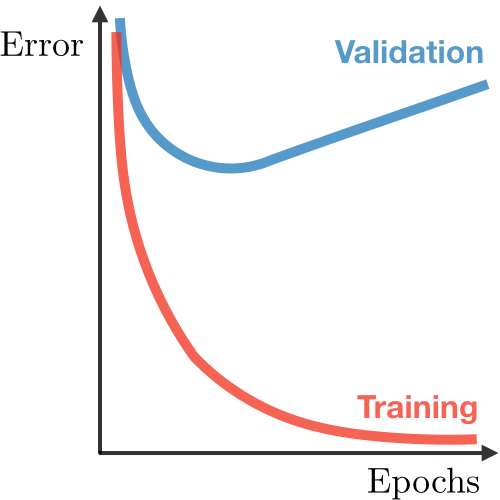
Number of Epochs - An epoch represents a full pass through the entire training dataset. Too few epochs might lead to underfitting, while too many can lead to overfitting. Finding the right number of epochs involves monitoring validation performance.
The k in k-nearest neighbors. The C and sigma hyperparameters for support vector machines.
Number of Layers: The number of layers in the neural network. This includes the input layer, hidden layers, and the output layer1.
Number of Nodes/Neurons: The number of nodes or neurons in each layer1.
Learning Rate: This controls how much to change the model in response to the estimated error each time the model weights are updated1.
Batch Size: The number of training examples utilized in one iteration1.
Number of Iterations: The number of epochs or the number of times the learning algorithm will work through the entire training dataset2.
Activation Function: The function used to transform the input signal into an output signal1.
Loss Function: The method of evaluating how well specific algorithm models the given data1.
Optimizer: The method used to adjust the attributes of the neural network such as weights and learning rate in order to reduce the losses1.
Dropout Rate: The proportion of neurons which are randomly selected to be ignored during training2.
Regularization Parameters: These parameters help to avoid overfitting2.
Momentum: This is a method that helps accelerate gradients vectors in the right directions, thus leading to faster converging2.
Weight Initialization Methods: The method or strategy used to set the initial random weights of neural networks2.
These hyperparameters play a crucial role in the performance of a neural network and they are usually tuned to optimize the performance1.
weight initialization methods used in neural networks. Here are some of the most common ones:
Zero Initialization: As the name suggests, all the weights are assigned zero as the initial value. This kind of initialization is highly ineffective as neurons learn the same feature during each iteration1.

Random Initialization: This assigns random values except for zeros as weights to neuron paths. However, assigning values randomly to the weights, problems such as Overfitting, Vanishing Gradient Problem, Exploding Gradient Problem might occur1. Random Initialization can be of two kinds:
    Random Normal: The weights are initialized from values in a normal distribution1.
    Random Uniform: The weights are initialized from values in a uniform distribution1.

Xavier/Glorot Initialization: This method initializes weights with a distribution based on the number of input and output neurons, providing a good starting point when the activation function is Sigmoid or Tanh2.

He Initialization: Similar to Xavier initialization, but it’s designed for layers with ReLU activation. It draws samples from a truncated normal distribution centered on 0 with sqrt(2/n) as the standard deviation, where n is the number of input units2.
These methods help in starting the training process from a point that’s not too far off from the optimal solution, speeding up convergence, and improving the final performance of the network12.
A model parameter is a configuration variable that is internal to the model and whose values are learned from training data.
Examples of model parameters include:
- The weights in an artificial neural network.
- The support vectors in a support vector machine.
- The coefficients in a linear regression or logistic regression.
What is the curse of dimensionality? Why do we need to reduce it? What is PCA, why is it helpful, and how does it work? What do eigenvalues and eigenvectors mean in PCA?
PCA stands for principal component analysis
- A dimensionality reduction technique
- ?
A method for assessing the performance of a model on unseen data by partitioning the dataset into training and validation sets multiple times, and averaging the evaluation metric across all partitions.
Can K-fold cross-validation be used on Time Series data? Explain with suitable reasons in support of your answer.
Time series cross-validation
There is a task called time series forecasting, which often arises in the form of “What will happen to the indicators of our product in the nearest day/month/year?”.
Cross-validation of models for such a task is complicated by the fact that the data should not overlap in time: the training data should come before the validation data, and the validation data should come before the test data. Taking into account these features, the folds in cross-validation for time series are arranged along the time axis as shown in the following image:
Cross-validation is a method used for evaluating the performance of a model, It helps to compare different models and select the best one for a specific task.
- Hold-out - The hold-out method is a simple division of data into train and test sets.
- Stratification - Simple random splitting of a dataset into training and test sets (as shown in the examples above) can lead to a situation where the distributions of the training and test sets are not the same as the original dataset. The class distribution in this dataset is uniform:
- 33.3% Setosa
- 33.3% Versicolor
- 33.3% Virginica
- k-Fold - The k-Fold method is often referred to when talking about cross-validation.
- Stratified k-Fold - The stratified k-Fold method is a k-Fold method that uses stratification when dividing into folds: each fold contains approximately the same class ratio as the entire original set.
K-fold cross-validation is a technique used in machine learning to assess the performance and generalization ability of a model. It helps us understand how well our model will perform on unseen data.
how K-fold cross-validation works:
- Splitting the dataset: First, you divide your dataset into K equal-sized subsets or folds. For example, let’s use K=5, so you’ll have 5 subsets, each containing 200 images.
- Training and testing: Now, you iterate through each fold, treating it as a testing set, while the remaining K-1 folds serve as the training set.
You are given a data set with missing values that spread along 1 standard deviation from the median. What percentage of data would remain unaffected?
The data is spread across the median, so we can assume we’re working with normal distribution. This means that approximately 68% of the data lies at 1 standard deviation from the mean. So, around 32% of the data is unaffected.
Data augmentation techniques are used to generate additional, synthetic data using the data you have.
NLP data augmentation methods provided in the following projects:
- Back translation.
- EDA (Easy Data Augmentation).
- NLP Albumentation.
- NLP Aug
Back translation - translate the text data to some language and then translate it back to the original language

EDA consists of four simple operations that do a surprisingly good job of preventing overfitting and helping train more robust models.
| Synonym Replacement | Random Insertion | Random Swap | Random Deletion |
|---|---|---|---|
| Randomly choose n words from the sentence that are not stop words. Replace each of these words with one of its synonyms chosen at random. | Find a random synonym of a random word in the sentence that is not a stop word. Insert that synonym into a random position in the sentence. Do this n times. | Randomly choose two words in the sentence and swap their positions. Do this n times. | Randomly remove each word in the sentence with probability p. |
| This article will focus on summarizing data augmentation techniques in NLP. This write-up will focus on summarizing data augmentation methods in NLP. |
This article will focus on summarizing data augmentation techniques in NLP. This article will focus on write-up summarizing data augmentation techniques in NLP methods. |
This article will focus on summarizing data augmentation techniques in NLP. This techniques will focus on summarizing data augmentation article in NLP. |
This article will focus on summarizing data augmentation techniques in NLP. This article focus on summarizing data augmentation in NLP. |
NLP Albumentation
- Shuffle Sentences Transform: In this transformation, if the given text sample contains multiple sentences these sentences are shuffled to create a new sample.
For example:
text = ‘<Sentence1>. <Sentence2>. <Sentence4>. <Sentence4>. <Sentence5>. <Sentence5>.’
Is transformed to:
text = ‘<Sentence2>. <Sentence3>. <Sentence1>. <Sentence5>. <Sentence5>. <Sentence4>.’
NLPAug Python Package helps you with augmenting NLP for your machine learning projects. NLPAug provides all the methods discussed above.
In computer vision applications data augmentations are done almost everywhere to get larger training data and make the model generalize better.
The main methods used involve:
- cropping,
- flipping,
- zooming,
- rotation,
- noise injection,
- and many others.
In computer vision, these transformations are done on the go using data generators.