Bias - the constant b of a linear function y = ax + b
- It allows you to move the line up and down to fit the prediction with the data better.
- Without b, the line always goes through the origin (0, 0) and you may get a poorer fit.
- A bias value allows you to shift the activation function to the left or right, which may be critical for successful learning.
The null hypothesis for a simple linear regression model is 𝐻0: 𝛽1=0
The strength of the linear regression model can be assessed using 2 metrics,
- R-Squared (R²) or Coefficient of Determination
- Residual Standard Error (RSE)
- R-Squared can take any value between 0 and 1
- Larger the R-squared value, the better the regression model fits the observations
RSS (Residual Sum of Squares) is defined as follows:
TSS(Total Sum of Squares) is defined as the sum of all squared differences between the observed dependent variable and its mean
- Linear Regression with NumPy - Using gradient descent to perform linear regression
- Linear Regression with Gradient Descent from Scratch
- Linear Regression from scratch (Gradient Descent)
- Gradient Descent From Scratch
- Multivariate Linear Regression from Scratch in Python
Logistic regression, by default, is limited to two-class classification problems. It can also be applied to multiclass problems.
- Logistic Regression: A Classifier With a Sense of Regression - Explaining logistic regression as a classifier derived from regression concept
- Multiclass Logistic Regression With Python
https://machinelearningmastery.com/intuition-for-bayes-theorem-with-worked-examples/
K-nearest neighbors (KNN) is a type of supervised learning algorithm used for both regression and classification. KNN tries to predict the correct class for the test data by calculating the distance between the test data and all the training points.
- Then select the K number of points which is closet to the test data.
- The KNN algorithm calculates the probability of the test data belonging to the classes of ‘K’ training data and class holds the highest probability will be selected.
- In the case of regression, the value is the mean of the ‘K’ selected training points.
'K' value indicates the count of the nearest neighbors. We have to compute distances between test points and trained labels points. Updating distance metrics with every iteration is computationally expensive, and that’s why KNN is a lazy learning algorithm.
There are various methods for calculating this distance, of which the most commonly known methods are,
| K-Nearest Neighbor Video Tutorial |
|---|
 |
Clustering is the task of grouping a set of objects, such that objects in the same group (cluster) are more similar to each other than to those in other groups (clusters).
K-means is a centroid-based clustering technique that partitions the dataset into k distinct clusters, where each data point belongs to the cluster with the nearest center.
K-means clustering is a widely-used unsupervised machine learning technique for data segmentation.
K-means can be employed for,
- Customer segmentation
- Image compression
- Document clustering
- and anomaly detection.
Centroid-Based Clustering
In centroid-based clustering, each cluster is represented by a central vector, called the cluster center or centroid, which is not necessarily a member of the dataset. The cluster centroid is typically defined as the mean of the points that belong to that cluster.
Our goal in centroid-based clustering is to divide the data points into k clusters in such a way that the points are as close as possible to the centroids of the clusters they belong to.
| K-Means Clustering Video Tutorial | Clustering with DBSCAN Video Tutorial |
|---|---|
 |
 |
The ways to select an optimal number of clusters (K) are,
Elbow Curve Method
- Perform K-means clustering with all these different values of K. For each of the K values, we calculate average distances to the centroid across all data points.
- Plot these points and find the point where the average distance from the centroid falls suddenly (“Elbow”).
- The elbow point can be used to determine K.
the elbow is at k=3 (i.e., the Sum of squared distances falls suddenly), indicating the optimal k for this dataset is 3.
Silhouette Score
The silhouette coefficient or silhouette score kmeans is a measure of how similar a data point is within-cluster (cohesion) compared to other clusters (separation).
- Select a range of values of k (say 1 to 10).
- Plot Silhouette coefficient for each value of K.
The equation for calculating the silhouette coefficient for a particular data point: silhouette score
We see that the silhouette score is maximized at k = 3. So, we will take 3 clusters.
Random Forest approach is an ensemble learning method based on many decision trees.
https://datagy.io/sklearn-random-forests/
-
A forest is made up of trees and these trees are randomly build.
-
Random Forests are often used for feature selection in a data science workflow.
-
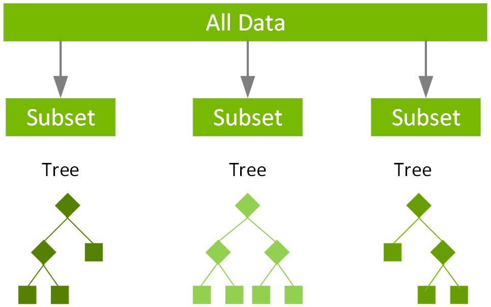
In random forest, decision trees are trained independent to each other.
-
The idea behind is a random forest is the automated handling of creating more decision trees. Each tree receives a vote in terms of how to classify. Some of these votes will be wildly overfitted and inaccurate. However, by creating a hundred trees the classification returned by the most trees is very likely to be the most accurate.
Classes, functions, and methods:
from sklearn.ensemble import RandomForestClassifier: random forest classifier from sklearn ensemble class.
plt.plot(x, y): draw line plot for the values of y against x values.
Random forest uses a technique called bagging to build full decision trees in parallel from random bootstrap samples of the data set. The final prediction is an average of all of the decision tree predictions.
In boosting, the trees are built sequentially such that each subsequent tree aims to reduce the errors of the previous tree. Each tree learns from its predecessors and updates the residual errors.
The term “gradient boosting” comes from the idea of “boosting” or improving a single weak model by combining it with a number of other weak models in order to generate a collectively strong model. Gradient boosting is an extension of boosting where the process of additively generating weak models is formalized as a gradient descent algorithm over an objective function.
Unlike Random Forest where each decision tree trains independently, in the Gradient Boosting Trees, the models are combined sequentially where each model takes the prediction errors made my the previous model and then tries to improve the prediction. This process continues to n number of iterations and in the end all the predictions get combined to make final prediction.
XGBoost stands for Extreme Gradient Boosting is an ensemble learning algorithm primarily based on gradient boosting and optimization principles.
- It builds a strong predictive model by combining the predictions of multiple weak learners, often decision trees, through an iterative process.
- It can be used both for regression and classification tasks.
The XGBoost algorithm consists of a series of decision trees that are trained sequentially. Each new tree is trained to correct the errors of the previous tree, gradually improving the model’s performance. The algorithm is called “gradient boosting” because it minimizes a loss function by iteratively adding new models that minimize the negative gradient of the loss function.
XGBoost is one of the libraries which implements the gradient boosting technique. To make use of the library, we need to install with pip install xgboost. To train and evaluate the model, we need to wrap our train and validation data into a special data structure from XGBoost which is called DMatrix. This data structure is optimized to train xgboost models faster.
xgb.train(): method to train xgboost model. xgb_params: key-value pairs of hyperparameters to train xgboost model. watchlist: list to store training and validation accuracy to evaluate the performance of the model after each training iteration. The list takes tuple of train and validation set from DMatrix wrapper, for example, watchlist = [(dtrain, 'train'), (dval, 'val')].
XGBoost, excel at handling tabular data for a multitude of reasons.
- First, their hierarchical structure is inherently adept at modeling the layered relationships often found in tabular formats.
- Second, they are particularly effective at automatically detecting and incorporating complex, non-linear interactions between features.
- Third, these algorithms are robust to the scale of input features, allowing them to perform well on raw datasets without the need for normalization.
Here’s a concise technical breakdown of how XGBoost works:
- Gradient Boosting: XGBoost follows a boosting approach where each new model corrects the errors of the previous ones, leading to incremental performance improvement.
- Loss Function: It minimizes a loss function that quantifies the disparity between predicted and actual values, using common loss functions such as mean squared error (for regression) and log loss (for classification).
- Gradient Descent: XGBoost employs gradient descent to minimize the loss function. It calculates the gradient of the loss concerning the current model’s predictions.
- Additive Learning: At each boosting iteration, a new decision tree (weak learner) is added to the ensemble. This tree aims to minimize the residual errors left by the previous trees.
- Weighted Updates: XGBoost assigns weights to data points, giving higher weights to those that are harder to predict (higher residual errors). This focuses the next model on rectifying these errors.
- Regularization: To prevent overfitting, XGBoost incorporates regularization terms (L1 and L2) that penalize complex models, encouraging simplicity.
- Learning Rate: It introduces a “learning rate” parameter controlling the step size of each iteration. A smaller rate slows learning, enabling finer adjustments.
- Feature Importance: XGBoost calculates feature importance scores by evaluating each feature’s contribution to reducing the loss function across all trees.
- Stopping Criteria: Training stops when predefined criteria are met, like a set number of trees or negligible loss improvement.
- Prediction: To make predictions, XGBoost combines the weak learners’ predictions, each scaled by a “shrinkage” factor (learning rate).
scikit-learn's XGBRegressor is an implementation of gradient boosting trees.
here are six (6) hyperparameters for XGBoost that are the most important , which is defined as those with the highest probability of the algorithm yielding the most accurate, unbiased results the quickest without over-fitting:
- (1) how many sub-trees to train;
- (2) the maximum tree depth (a regularization hyperparameter);
- (3) the learning rate;
- (4) the L1 (reg_alpha) and L2 (reg_ lambda) regularization rates that determine the extremity of weights on the leaves;
- (5) the complexity control (gamma=γ), a pseudo- regularization hyperparameter; and
- (6) minimum child weight, another regularization hyperparameter.
- In 2D data, a Support Vector Classifier is a line.
- In 3D, it is a plane.
- In 4 or more dimensions, Support Vector Classifier is a hyperplane.
Technically all SVCs are a hyperplane, but it is easier to call them planes in the case of 2D.
 |
 |
Important concepts in SVM which will be used frequently are as follows.
- Hyperplane − It is a decision plane or space which is divided between a set of objects having different classes.
- Support Vectors − Datapoints that are closest to the hyperplane are called support vectors. The separating line will be defined with the help of these data points.
- Kernel — A kernel is a function used in SVM for helping to solve problems. They provide shortcuts to avoid complex calculations.
- Margin − It may be defined as the gap between two lines on the closet data points of different classes. A large margin is considered a good margin and a small margin is considered as a bad margin.
Support Vector Machines use Kernal Functions to find Support Vector Classifiers in higher dimensions. A kernel function is a function that takes two input data points in the original input space and calculates the inner product of their corresponding feature vectors in a transformed (higher-dimensional) feature space.
| Polynomial Kernel | Radial Kernel (RBF) |
|---|---|
| The polynomial kernel is used to transform the input data from a lower-dimensional space to a higher-dimensional space where it is easier to separate the classes using a linear decision boundary. | Radial Kernel finds Support Vector Classifiers in infinite dimensions. It assigns a higher weight to points closer to the test point and a lower weight to points farther away (like nearest neighbors). Observations that further away have relatively little influence on the classification of a data point. |
In general, SVMs are suitable for classification tasks where the number of features is relatively small compared to the number of samples, and where there is a clear margin of separation between the different classes. SVMs can also handle high-dimensional data and nonlinear relationships between the features and the target variable. However, SVMs may not be suitable for very large datasets, as they can be computationally intensive and require a lot of memory.


