Convolutional Neural Networks are built stacking a series of these layers shown below in specific manner.
- Convolutional (CONV) Layers
- Activation (ACT or RELU, where we use the same or the actual activation function)
- Pooling (POOL) Lyer
- Fully connected (FC)
- Batch normalization (BN)
- Dropout (DO)
- Convolution operation in CNNs is to extract features from the input image or feature map by applying different filters to an input image, the network can identify edges, lines, curves, and textures that are important for recognition tasks.
- Convolution uses a ‘kernel’ or 'filters' or ' feature detectors' to extract certain ‘features’ from an input image.
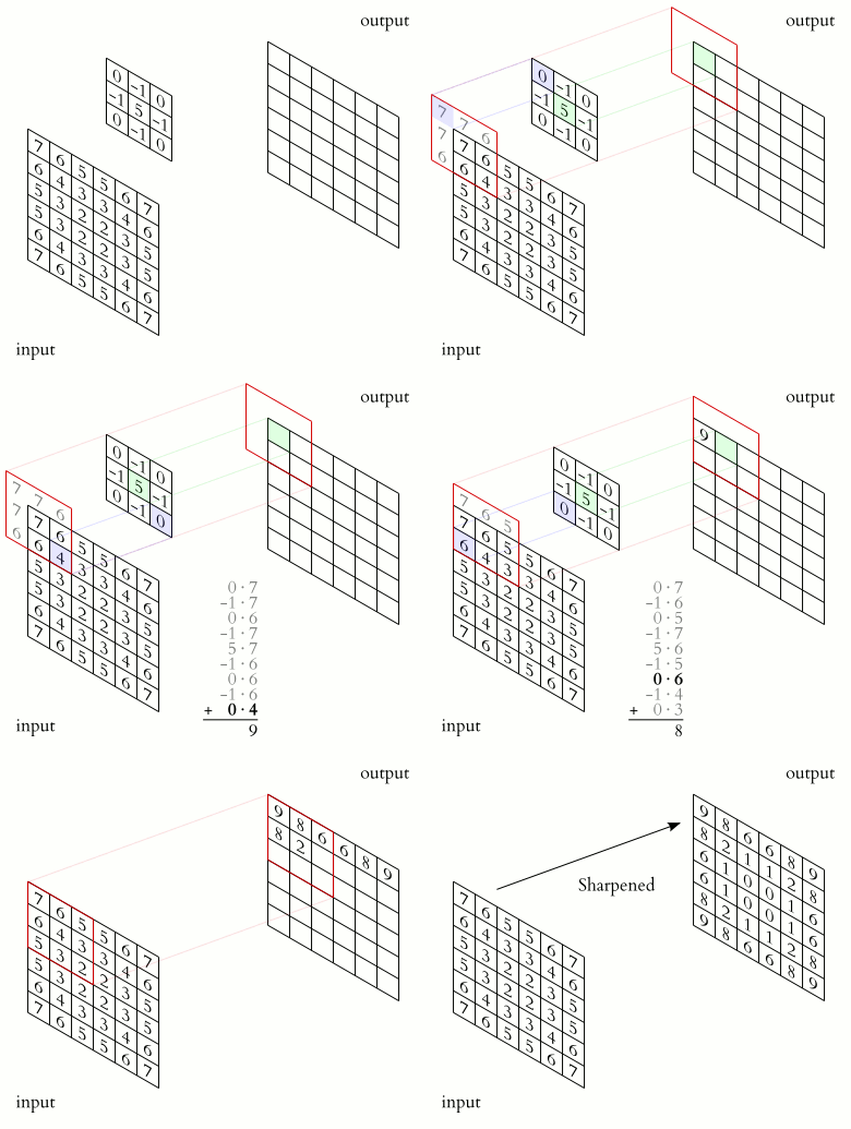
- The convolutional operation is implemented by making The 'kernel' or 'filter' slides across the image and produces an output Value at each position.
- Convolutional layers can learn to recognize low-level features such as edges and corners, and then combine them to detect more complex features such as shapes and patterns.
- A kernel is a matrix, which is slid across the image and multiplied with the input such that the output is enhanced in a certain desirable manner.
- Also we convolve different Kernels and as a result obtain Different feature maps or channels. to extract latent features.
The kernel animation for sharpening the image is shown below,
In CNNs, a feature map is the output of a convolutional layer representing specific features in the input image or feature map.
Take an input FloatTensor with torch.Size = [10, 3, 28, 28] in NCHW order, and apply nn.Conv2d(in_channels=3, out_channels=16, kernel_size=(5,5), stride=(1,1), padding=(0,0))
in channels cin = 3 out channels cout = 16 number of filters f = 16 size of filters k = 5 stride s = 1 padding p = 0 height in h = 28 width in w = 28
The formula used to calculate the output shape is:
output_shape = ((input_height - kernel_size + 2 * padding) / stride) + 1 = ((28 - 5 + 2 * 1)/(1) + 1) = 24
Output shape: 24 x 24 x 16
Conv2D calculator: https://abdumhmd.github.io/files/conv2d.html
- http://layer-calc.com/
- https://ravivaishnav20.medium.com/visualizing-feature-maps-using-pytorch-12a48cd1e573
Pooling layers are used to reduce the spatial dimensions of feature maps generated by the convolutional layers. This process helps in reducing the computational complexity of the network and prevents overfitting.
The most common pooling operation is max-pooling, which takes the maximum value from a defined region (usually 2×2 or 3×3) of the feature map.
A pooling function replaces the output of the net at a certain location with a summary statistic of the nearby outputs. For example,
- Max pooling operation reports the maximum output within a rectangular neighborhood.
- Others,
- Average of a rectangular neighborhood
- L2 norm of a rectangular neighborhood
- A weighted average based on the distance from the central pixel.
In all cases, pooling helps to make the representation become approximately invariant to small translations of the input. Invariance to translation means that if we translate the input by a small amount, the values of most of the pooled outputs do not change.
Pooling is then applied over the feature maps for invariance to translation.
- Since pooling takes a statistical aggregate over multiple regions of an image, it makes the network invariant to 'local transformations' (such as the face being tilted a little, or an object being located in a different region than what the training data had seen).
- Pooling reduces the number of parameters and computation, it also controls overfitting.
- Pooling reduces the width and height, thereby reducing the number of parameters and the amount of computation (since with less number of parameters there will be fewer computations involved in feedforward/backpropagation etc.).
Understanding the Receptive Field of Convolutional Layer
For large inputs, we need many layers to understand the whole input. We can downsample the features by using stride, kernel_size and max_pooling. They increase the receptive field. The receptive field essentially expresses how much information a later layer contains of the first input layer. Consider the example of a 1D array of length 7, where we apply a 1D kernel of size 3. On the left we see that the 1D array length decreases from 7 to 5 in the second layer due to the convolutional operation.


