Image Recognition At Pixel Level By Artificial Intelligence: One Step Toward Automatic Seismic Interpretation
In this two-week Capstone project, I built a deep learning model for image recognition at pixel level (semantic segmentation) that slightly beat MIT baseline model by 1% in pixel accuracy and 4% in mean IoU. This algorithm has great potential to be applied in oil and gas industry to achieve truely automatic seismic image interpretation.
Semantic segmentation is a very active forfront research area in deep learning. I studied and assessed several state of art neural network structures in different deep learning frameworks, including tensorflow, pytorch, and keras, and selected PSPNET for my capstone project. I implemented the PSPNET in keras/tensorflow, and trained the final model on top of the pre-trained model.
For less techinical audience, here is my presentation. If you want to know details, please keep reading.
If you want to make a quick experiment on your own data, I have a web app in app/ folder. It can be host on AWS EC2 g3 instances. Author's contact: [email protected]
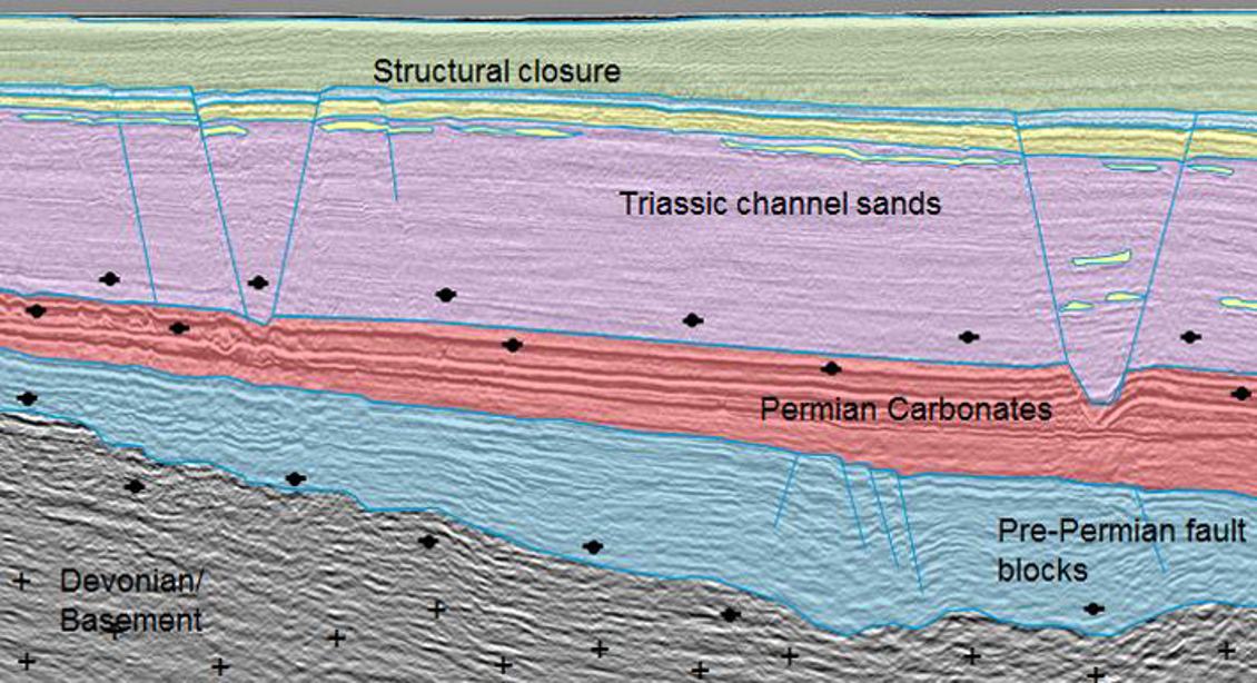
Where to drill and when to drill is one of the most important items on stake holder worry plate in oil and gas E&P. A well interpreted seismic image is an important tool on the table to help answer those questions. Interpreting a seismic image requires that the interpreter manually check the seismic image and draw upon his or her geological understanding to pick the most likely interpretation from the many “valid” interpretations that the data allow.
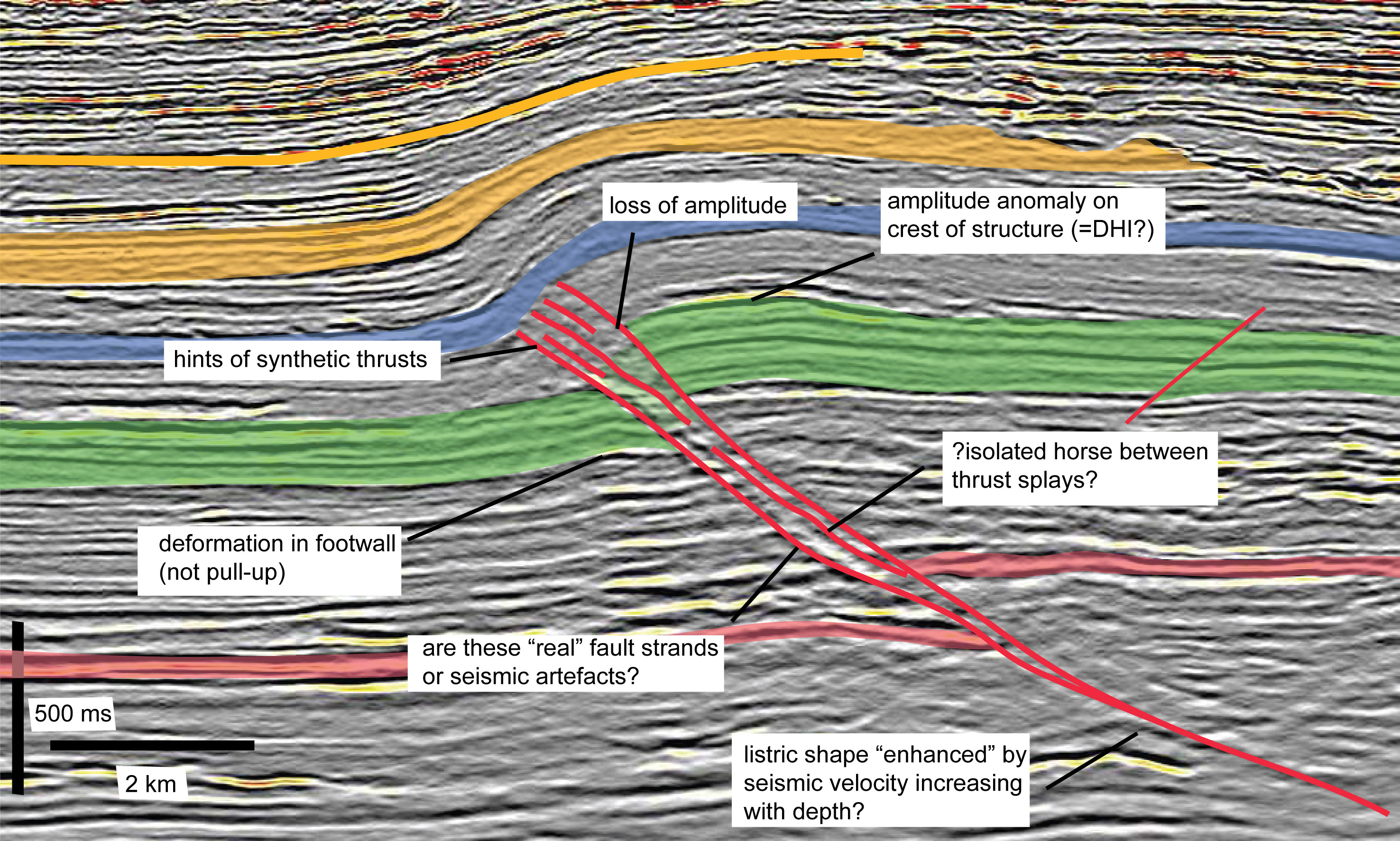
Interpreting faults in seismic image is difficult and tedious, especially in complex, highly faulted formations. Faults can be difficult to pick if they are steeply dipping, or if they are aligned such that they are not easily visible on Inlines or Crosslines. Inaccurate and incomplete interpretations often lead to missed pay, inefficient field development, miscorrelations, drilling hazards – and ultimately dry holes.There are many state-of-art solutions to speed up the process, these solutions fall in the region of feature engineering and hard to generalize. The current best practice is still semi-automatic or hand-picking by human experts.
Why deep learning? Deep learning provides a paradigm for a true automatic seismic interpretation. Unlike traditional feature engineering, deep learning integrates information from the interpreted(labled) seismic images in all the legacy projects and learns the features that best describe geological information in its deeper layers. Instead of repetative hand-picking and correction from scratch in each project, it constantly improves quality by learning from new projects.
The challenges for a sucessful deep learning project are datasets and algorithms. For seismic interpretation, most of the interpreted data sets are proprietary assets of big oil companies, and it is not publicly available to deep learning community. The deep learning research in seismic exploration community is sitll in the early stage. Because the unique requirement of seismic interpretation, there is still no concensus which algorithm has good/best performance.
| Seismic Interpretation | Semantic Segmentation |
|---|---|
 |
 |
Semantic segmentation is potentially a good Deep Learning solution to seismic Falut/Horizon picking and interpretation as they share many common challenges: 1. Pixel level accuracy. 2. Pixel level classification: in semantic segmentation, we identify each pixel as car, pedestrain and in seismic fault/horizon interpretation, we identify pixel as layers between Petrel and Oligocence or in a Fault block...
In this capstone project, I will focus on the algorithm part of the deep learning challenges. I will assess several state-of-art algorithms for semantic segmentations that are public available.
In this project, I choose ADE20K Dataset, which was released by MIT as the data sets for MIT Scene Parsing chanllenges (2017). The ADE20k data set contains more than 20K scene-centric images exhaustively annotated with objects and object parts. Specifically, the benchmark is divided into 20K images for training, 2K images for validation, and another batch of held-out images for testing. There are totally 150 semantic categories included in the challenge for evaluation, which include stuffs like sky, road, grass, and discrete objects like person, car, bed.
 |
 |
|---|---|
| Raw Images | Annotation |

In my capstone project, I choose AWS EC2 GPU instances for my model building, because all the state of arts semantic segmentation alogrithms are built on neural networks with very deep layers, and training on the modern GPU-acclerated machines drastically speed up the model building process (> 100 times faster). Both single GPUs and multiple parallel GPUs options were used depending on the model and memory requirement.
For the deep learning frameworks, I choose the current most popular frameworks including tensorflow, keras and pytorch. For for model prototyping and improvement, I used keras and tensorflow, and for assessing the state of arts algorithms I used pytorch as well, as some of the models are more accessible in pytorch.
MIT provides a benchmark model in pytorch for their scene parsing competition, which I will use as my benchmark model for model assessment.
To assess performance, we use two metrics:
(1) mean of pixel wise accuracy.

(2) Mean of the standard Jaccard Index, commonly known as the PASCAL VOC intersection-over-union metric IoU=TP/TP+FP+FN, where TP, FP, and FN are the numbers of true positive, false positive, and false negative pixels, respectively, determined over the whole test set.
To evalute your own prediction, run the code as follows. In order to make cross-platform cross-framework comparison, we saved all the predicted images as numpy array in .npy format.
python src/metrics_acc_iou.py --List_predict List_Prediction --List_true List_validation --num_class 10
Image annotation quality is checked and I randomly selected 40 pictures and put the raw image and annotation image in togglable slides in a PPT. Overall the quality of the annotation is very good for this assessement.
Seismic images only have one value in a pixel, compared to the RGB color scale in the training data sets. In this project, I used the RGB colored images. In the rest of this section, I will assess how much impact of gray image on the performance of Deep Learning using MIT baseline model. Gleam algorithm was found to be almost always the top performer for face and object recognition. Gleam method uses standard gamma correction on RGB channels, and takes the mean of the corrected RGB channels as grayscale intensity.
 where
where ![]()
![]()
![]() are gamma corrected RGB channels.
are gamma corrected RGB channels.
I trained a the MIT baseline model (Resnet34 with dillated modification + billinear decoder) on both RGB and Gray scale images for 5 iterations (~ 90 % of the performance are achieved in the first 5 iterations), and assessed their performance at predicting the 2000 validation images. Based on the observation, the performance of deep neural networks trained on gray image is only ~ 1% worse than that trained on RGB image, and most of the predicting power between the two models are the same. So the deep neural network structure is adaptitable to gray images such as seismic images.
| Pixel_Accuracy | Mean IOU | |
|---|---|---|
| RGB Image | 0.7498 | 0.296 |
| Gray Image | 0.7366 | 0.278 |
Raw Image/Annotations/Predicted


ImageNet is an image database organized according to the WordNet hierarchy (currently only the nouns), in which each node of the hierarchy is depicted by hundreds and thousands of images. There are more than 14 million labeled pictures for more than 22,000 categories available for free on ImageNet. In the context of ImageNet, sometimes people refer to several recognized high-performance deep learning structures trained on ImageNet dataset for image classification, including VGG, ResNet, Inception, and Xception. Those high-performance structures and the pre-trained weights are very popluar as a starting point for many other image recognition application. In this project, I investigated several structures for semantic segmentation that use Resnet as their starting point.

Another main challenge for segmentations using convolutional neural network is the pooling layer, which increase the field of view and aggregate the information from a larger context at the expenses of losing the resolution. However, semantic segmentation requires pixel level accuray for predicting the labels. One of the popular structures for semantic segnmentation is the encoder-decoder, in which encoder gradually reduces the spatial resolution with pooling layer while decoder gradually recovers the spatial resolution and details of the object. Another useful layer structure for keeping the spatial resolution is dilated/atrous convolution layer, in which the convolution kernel is dilated by a ratio, e.g. 2x, 4x, or 8x. This dilated convolution is able to aggreate information from larger field of view and lose less spatial information.

| Ordinary Convolution | Dilated Convolution |
|---|---|
 |
 |
Most state of art semantic segmentation deep learning architectures are based on these key components, with different flavors of implementation, training, data augmentation and post-processing.
MIT Baseline Model (Pytorch (resnet34_dilated8 + C1_bilinear))
MIT hosts a Scene Parsing Chanllenge in 2016 to segment and parse an image into different image regions associated with semantic categories, such as sky, road, person, and bed. The participants are from many famous universities and companies all over the world. In the end of 2017, they released a benchmark model and pre-trained model that includes many state of art deep learning architecture for semantic segmentation from the challenges. As a baseline model, I selected the ResNet34 with dilation modification as encoder, and C1_bilinar model as decoder. The reported score for this model has mean IoU of 0.327, and accuracy of 76.47%. The best performance from MIT baseline model options has mean IoU of 0.38, and accuracy of 78.21%.
Piramid Scence Parsing Network (Tensorflow, Caffe)
The piramid scence parsing module was in the champion model of MIT Scene Parsing Challenge 2016, which was able to aggreagate the information of pictures with different scale of views and thus leads to better prediction for the hard scene context. As shown in the picture below, the author selected four scales 1, 2, 3, 6 to aggregate the feature information, and then upsampling and stack the results. I used exact the same module in my project.

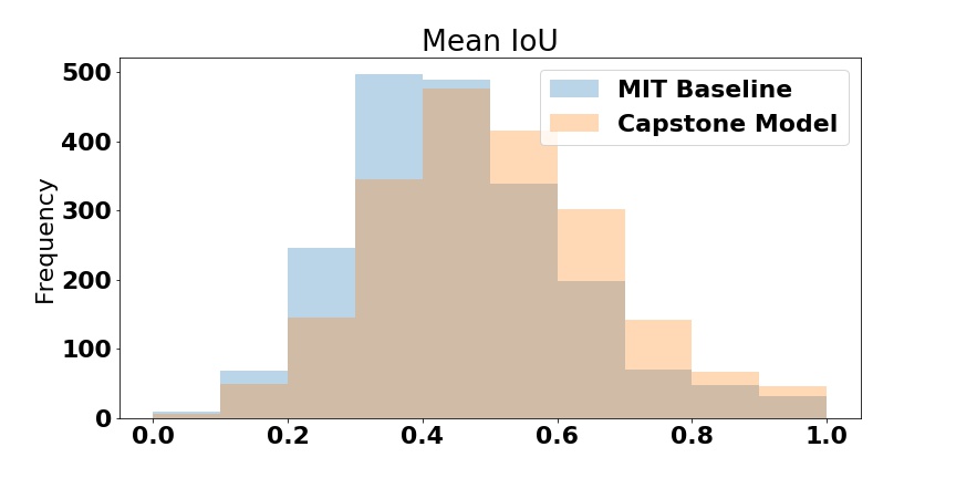
We used the 2000 labeled validation pictures to assess the perfomance of my Capstone model and MIT baseline model. The detailed layers and operations in these two models can be found in the tables. (MITBASELINE Capstone Model)
Both models worked very well, and my Capstone model has several additional features that contributed to the improvement over MIT baseline model: 1. Deeper resnets 50 vs 34; 2. PSP Module helps aggreate global context information better. 3. Flipped prediction vs non-flipped prediction; 4. Nonlinear upsampling method Cubic vs Bilinear.
| Model | Important Strucutre and Features | Mean Pixel Accuracy | Mean IoU |
|---|---|---|---|
| MIT Baseline Model | ResNet34 + Billinear Upsampling + Multi-scale Prediction | 0.7805 | 0.360 |
| Capstone Model | ResNet50 + PSP Module + Cubic Upsampling + Multi-scale and Flipped Prediction | 0.7951 | 0.406 |
 |
|---|
Beyond the numbers and statistics, I show a few predicton examples of images to have a better idea of how the models performed.
Example 1. Capstone model is able to handle confusing labels better than MIT Baseline Model. In this case, building and house are very close and it is even hard for a human being to differentiate from the two.

Example 2. Capstone model is able to learn and identify object not even labeled by human experts. In this case, the river is not labeled in the human label, but the deep learning model learned from other "experiences" and was able to delinear the river object correctly.

In this capstone project, I trained a deep learning model (PSPNET) for image recognition at pixel level that performes slightly better than MIT baseline model. The deep learning algorithm has great potential to achieve real automatic image interpretation/delineation. With enough training samples, the deep learning algorith is able to differentiate subtle difference of objects and catch the ignored object by human experts.
Several challenges that we need to tackle in the future:
- High-resultion: Our current deep learning implementation compress the image to 1/8 or even more of the original size, rely on interpolation algorithm to recover. Some of the resolutions are lost in the process.
- Memory constraints: training a deep nets with high-resolution image in the pipeline consumes a significant amount of memory. For a typical GPU of 8 GB mem and input image size of 481 x 481, training a deep nets only allows 2 pictures in a batch.
The two challenges above require a significant change and experiment on top of the current network structure. There is another structure proposed by Facebook AI research (mask RCNN) that is worth to test in the future.
- Data sets: A good quality data sets in each applicatoin domain is essential
AWS EC2 g3x4 Large instance has almost all the packages and resource needed to train the Neural Nets in this project. The enviroment is tensorflow_p36.
Code folders
- model/ source code for deep learning model
- src/ helper function for visulization, prediction metrics, and quality control
To convert images from RGB to grayscale, run the code as follows,
python src/rgb2gray.py  --input_folder INPUT_FOLDER --output_folder OUTPUT_FOLDER

options: --method (“luminance”,”gleam“)
To predict labels with your own image. Note that the output file is a .npy file which contains a 2d array of predictions
python models/pspnet_train.py --input_list LIST_OF_IMAGE.txt --output_path FOLDER_TO_SAVE_PREDICTION --weights MODEL_WEIGHTS_FOR_PREDICTION
To train a neural network. Note, the training is very slow based on current implementation. For 20k images, it takes 5 hours for 1 iteration on AWS EC2 g3.4xlarge. I recommend not to train from scratch.
python models/pspnet_train.py -train LIST_TRAIN_IMAGE.txt -lab LIST_LABEL_IMAGE.txt --weights PRE_TRAINED_WEIGHT_TO_START --num_epoch NUM_ITER --learning_rate 0.00001 --optimizer SGD
To assess a prediction results, we calculate Pixel level accuracy and IoU,
python src/metrics_acc_iou.py --List_predict LIST_OF_PREDICTION_NPY --List_true LIST_OF_HUMAN_LABEL --num_class 150
To visualize the predicted image and compared to human label,
python src/concat_image.py --image_predict LIST_OF_PREDICTION_NPY
I refered to two repos for this project.
- A 2017 Guide to Semantic Segmentation with Deep Learning
- Scene Parsing through ADE20K Dataset. Bolei Zhou, Hang Zhao, Xavier Puig, Sanja Fidler, Adela Barriuso and Antonio Torralba. Computer Vision and Pattern Recognition (CVPR), 2017.
- Semantic Understanding of Scenes through ADE20K Dataset. Bolei Zhou, Hang Zhao, Xavier Puig, Sanja Fidler, Adela Barriuso and Antonio Torralba. arXiv:1608.05442.
- Pyramid Scene Parsing Network
- Color-to-Grayscale: Does the Method Matter in Image Recognition?
- The Cityscapes Dataset for Semantic Urban Scene Understanding
- Hands Deep in Deep Learning for Hand Pose Estimation