Home
HNN-UI can be used from your web browser without the need to install anything on your local system. A test deployment is currently available here, note that this has a limited number of simultaneous users, so if it is busy please try again at a later time. Alternatively HNN-UI can also be installed on your local system using a pre-packaged Docker container.
HNN (https://hnn.brown.edu/) is a user-friendly software tool that gives researchers and clinicians the ability to test and develop hypotheses on the circuit mechanism underlying their EEG/MEG data in an easy-to-use environment. The foundation of HNN is a computational neural model that simulates the electrical activity of the neocortical cells and circuits that generate the primary electrical currents underlying EEG/MEG recordings.
Note: HNN UI is currently in development and the version you are using is an alpha release. Some functionality might not behave as expected. If you have problems please open a new issue.
The UI splits the workflows in two tabs available at the top of the screen: Run simulation and Set parameters.
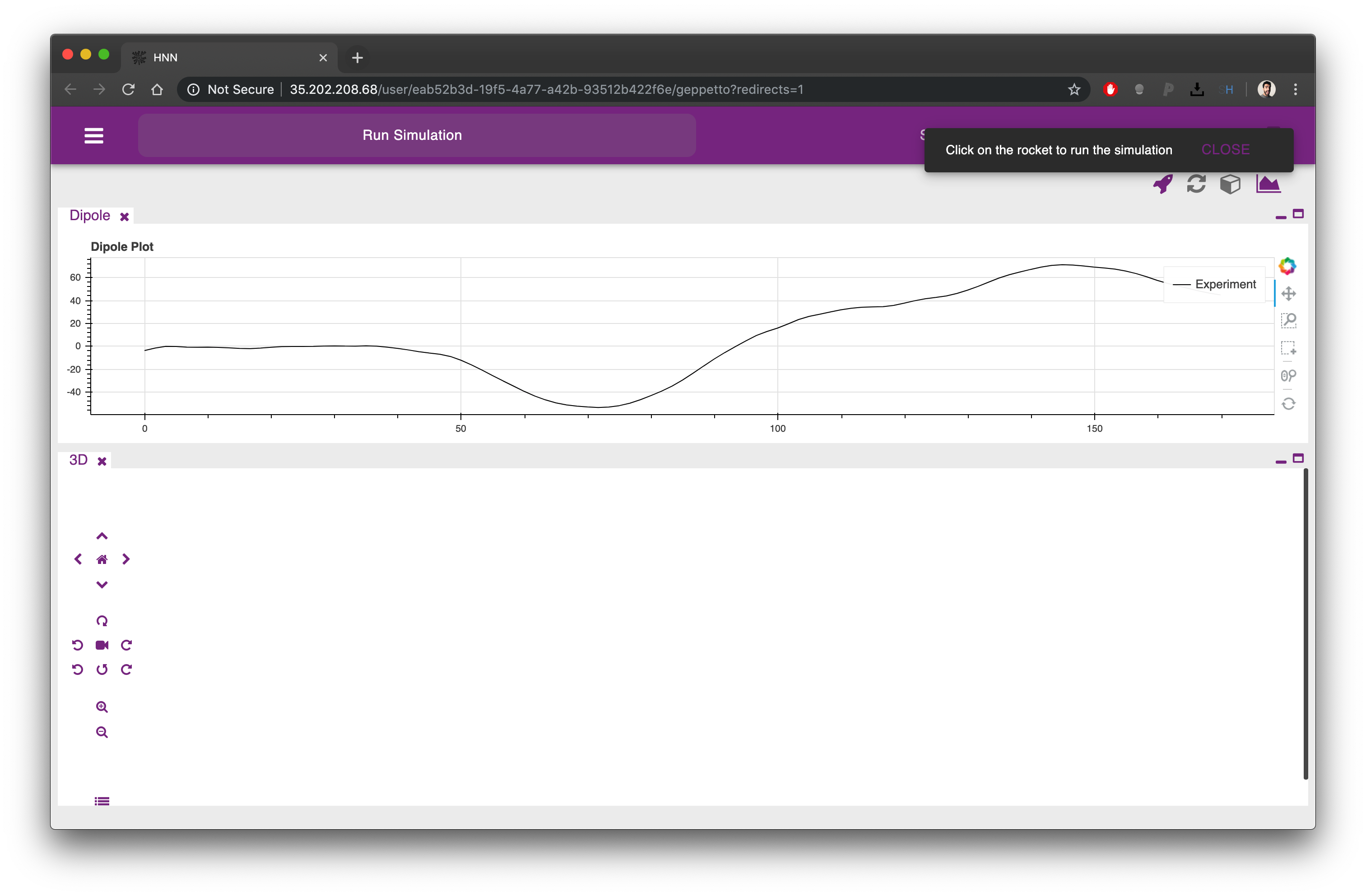
From the first tab it is possible to simulate the HNN model clicking on the rocket icon on the top right corner of the UI. The Dipole plot is open by default, at the top of the screen, conveniently showing an experimental trace that we will be able to compare as a reference to the result of our simulation.
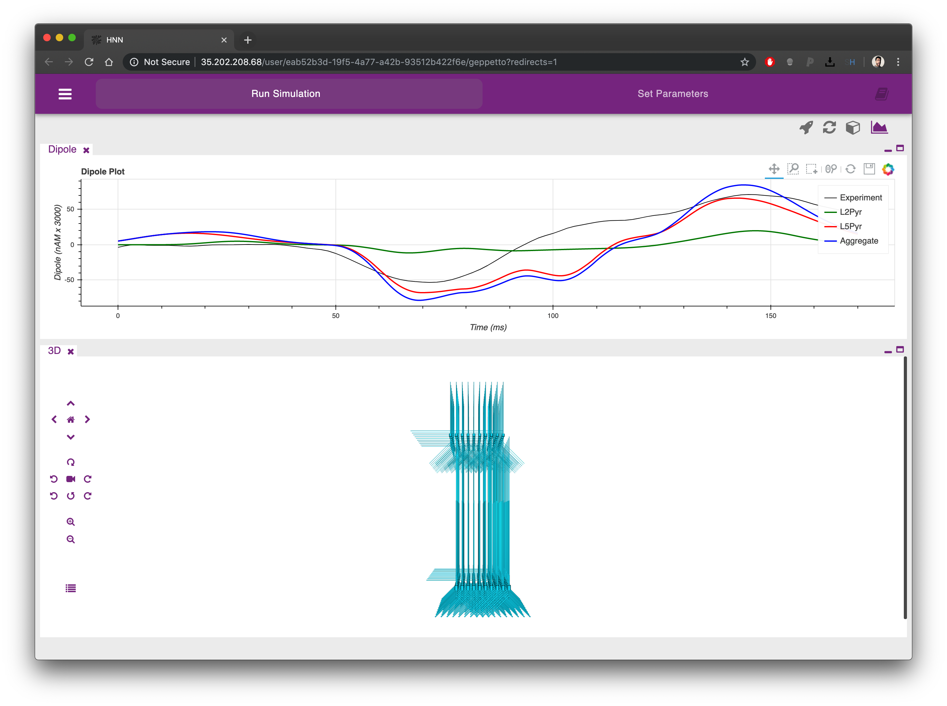
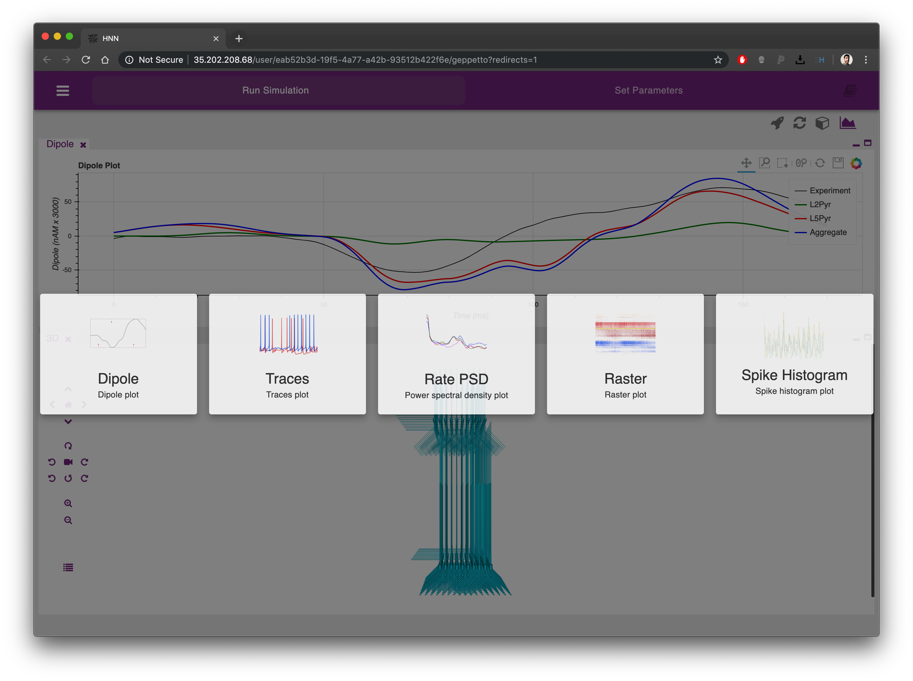
Once the simulation is completed (one to few minutes depending on the simulation parameters) you will see the Dipole plot populated with additional traces coming from the simulation you just executed. Using the plot menu (the first icon from the right at the top) you can choose among a range of available plots to analyse your model.
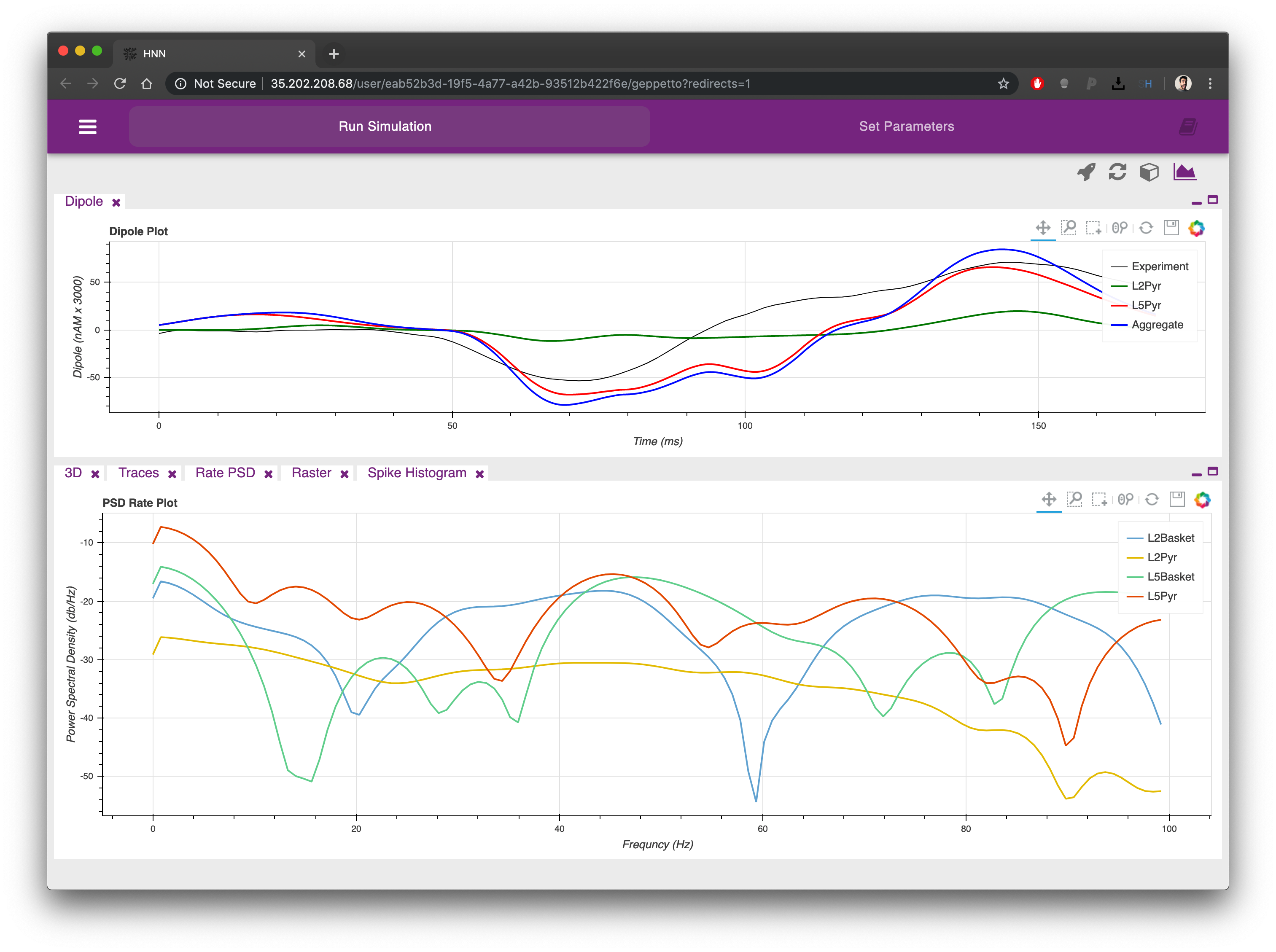
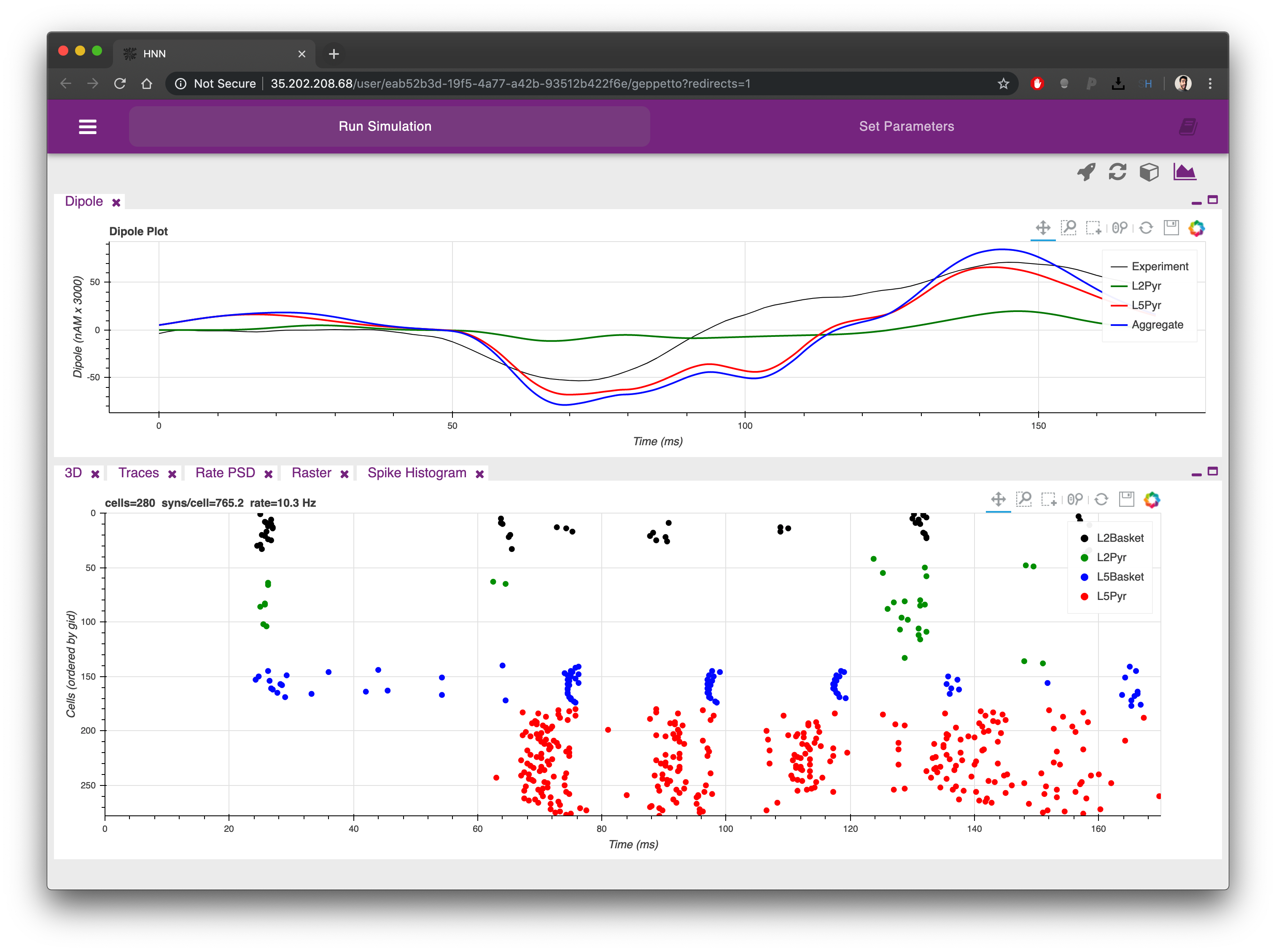
The plots can be re-arranged on the screen simply clicking on their labels and dragging them in a different position. Each plot can also be minimized and maximized using the icons on the top right corner of each.

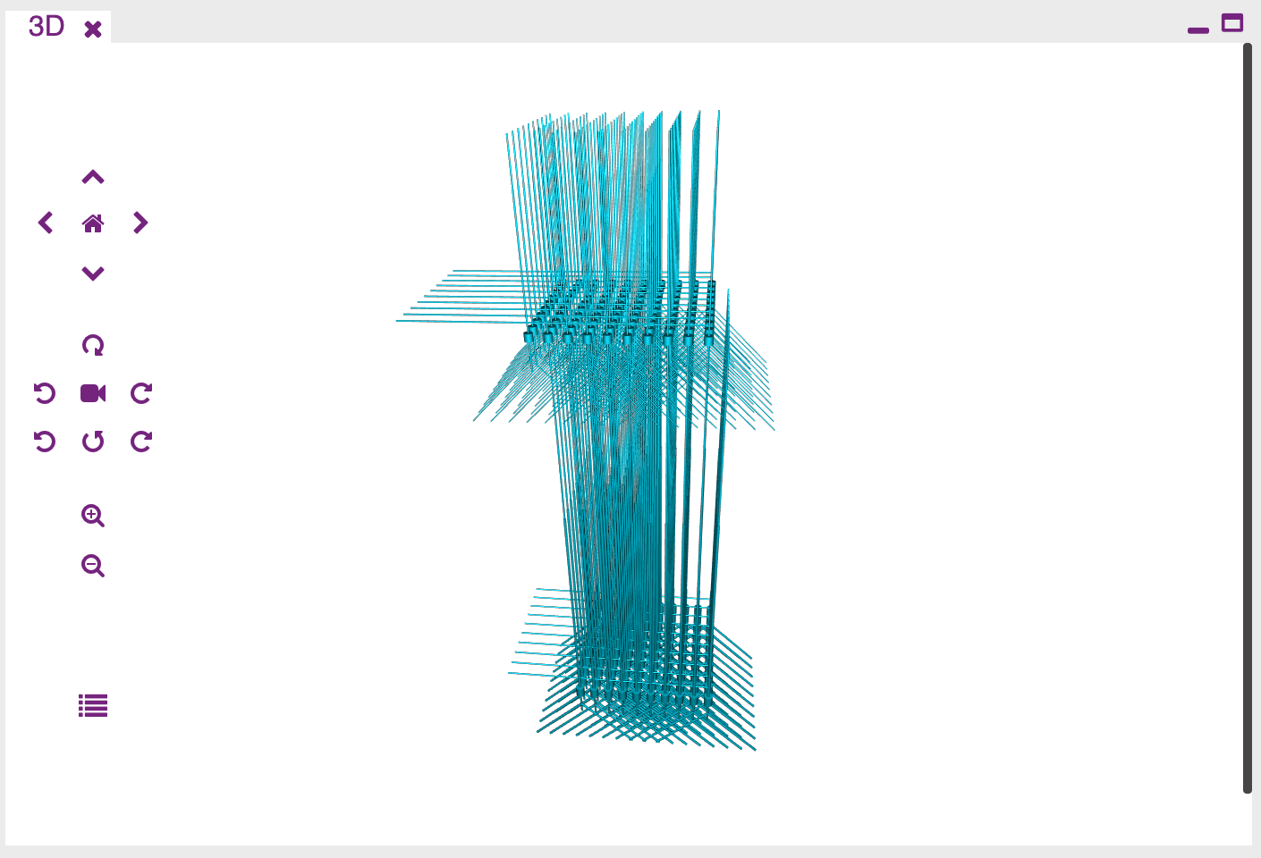
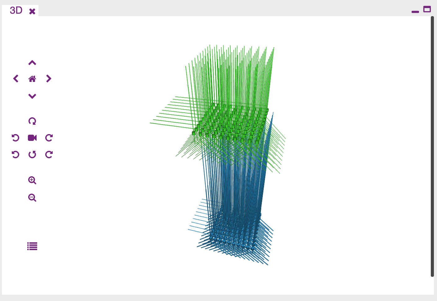
From the 3D Canvas window (opened by default, second icon from the right at the top) it is possible to inspect the morphologies of the simulated network:
The icon at the bottom inside the 3D canvas will let you open a control panel to inspect in a tabular form all the populations and single cells that were created from the HNN model definition.
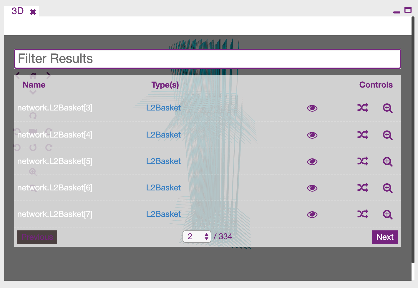
For each cell or population you can (in order) show or hide the element, change its colour, assign a random one, or zoom.
From the second tab it is possible to define the network and all the rules that will be used for its generation. Network definition comprises 7 different sections:
- Cell parameters
- Network parameters
- Input parameters
- Simulation parameters

Once you have changed the parameters of your model you can click on the first tab to simulate it again. The results of the previous simulation will be overwritten.
Clicking on the icon on the top left corner from each tab it is possible to open the AppBar
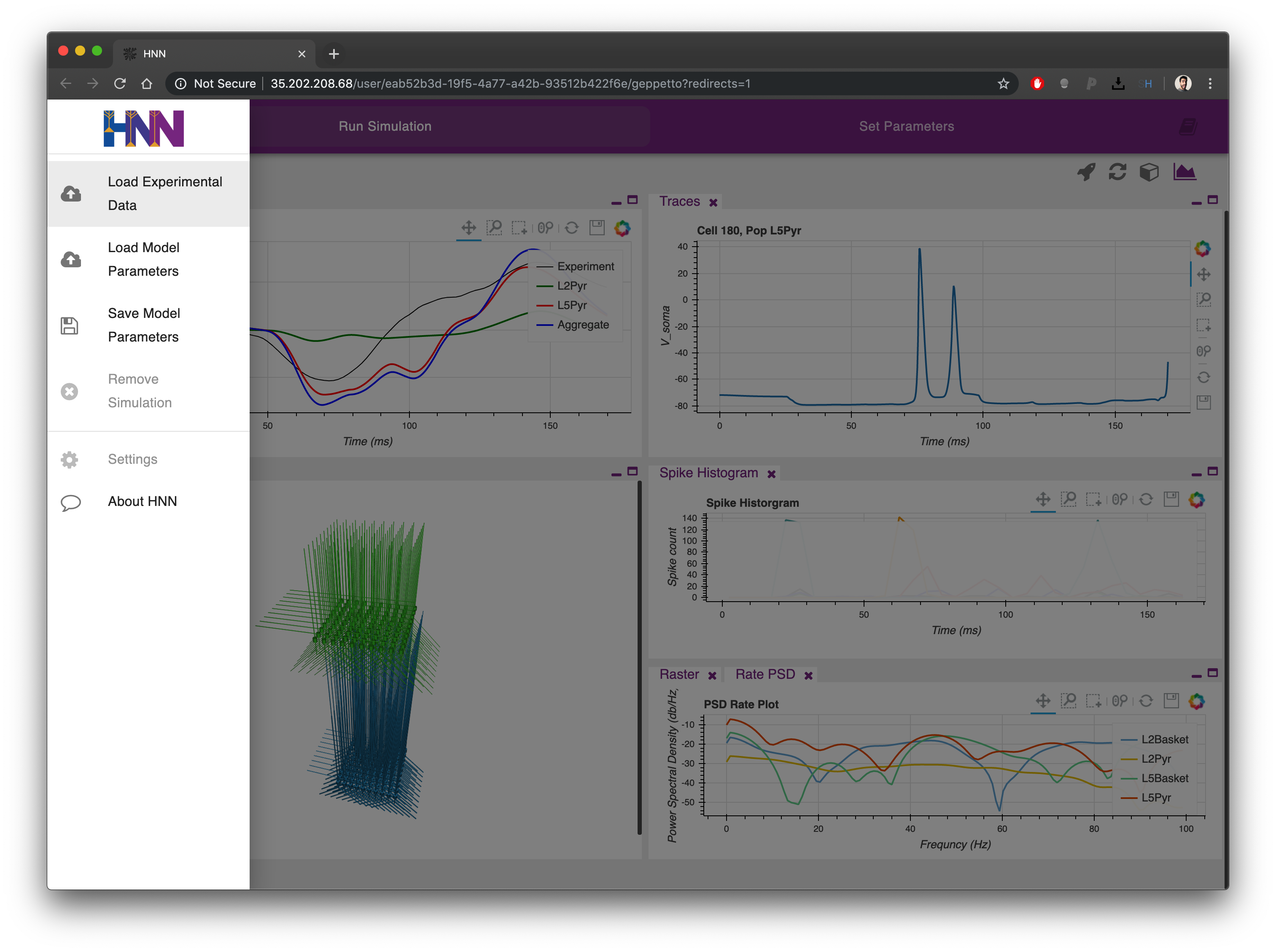
From the AppBar these options are available:
- Load Experimental Data : Load a new experimental trace for the Dipole plot window. This will replace the previous plot. The format is a txt file with two columns (sample here)
- Load Model Parameters : Load from file a set of previously saved parameters for the model. This will replace the parameters in the second tab.
- Save Model Parameters : Save to file the parameters currently present in the second tab.