DYffusion: A Dynamics-informed Diffusion Model for Spatiotemporal Forecasting (NeurIPS 2023)

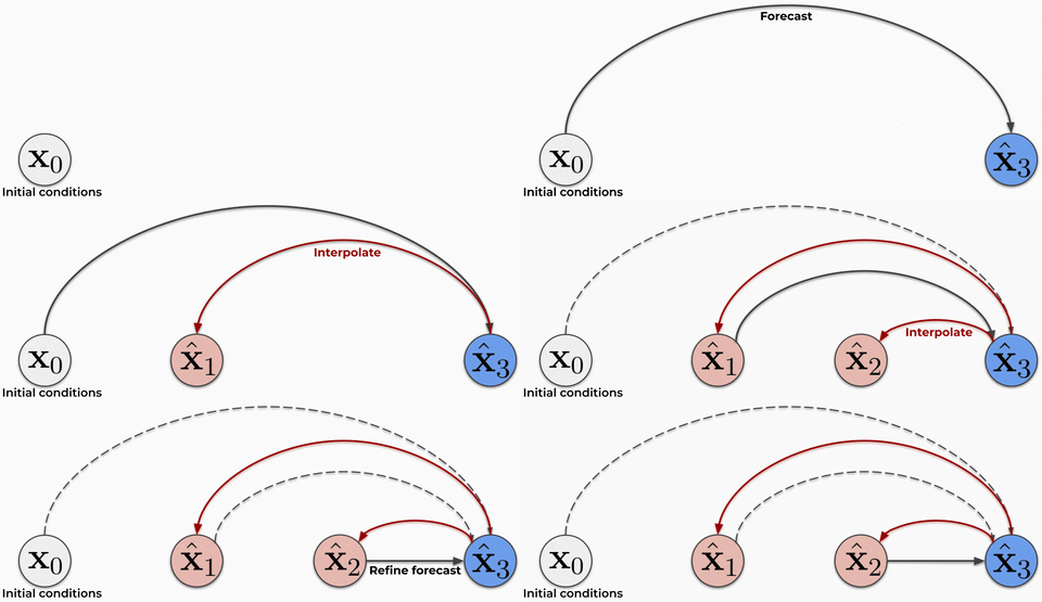
✨Official implementation of our DYffusion paper✨

DYffusion forecasts a sequence of $h$ snapshots $\mathbf{x}_1, \mathbf{x}_2, \dots, \mathbf{x}_h$ given the initial conditions $\mathbf{x}_0$ similarly to how standard diffusion models are used to sample from a distribution.

If you use this code, please consider citing our work. Copy the bibtex from the bottom of this Readme or cite as:

DYffusion: A Dynamics-informed Diffusion Model for Spatiotemporal Forecasting,
Salva Rühling Cachay, Bo Zhao, Hailey Joren, and Rose Yu,
Advances in Neural Information Processing Systems (NeurIPS), 2023

| Environment Setup

We recommend installing dyffusion in a virtual environment from PyPi or Conda. For more details about installing PyTorch, please refer to their official documentation. For some compute setups you may want to install pytorch first for proper GPU support.

python3 -m pip install ".[train]"

| Downloading Data

Navier-Stokes and spring mesh: Follow the instructions given by the original dataset paper. Or, simply run our scripts to download the data. For Navier-Stokes: bash scripts/download_navier_stokes.sh. For spring mesh: bash scripts/download_spring_mesh.sh.

By default, the data are downloaded to $HOME/data/physical-nn-benchmark, you can override this by setting the DATA_DIR in the scripts/download_physical_systems_data.sh script.

Sea surface temperatures: Pre-processed SST data can be downloaded from Zenodo: https://zenodo.org/record/7259555

IMPORTANT: By default, our code expects the data to be in the $HOME/data/physical-nn-benchmark and $HOME/data/oisstv2 directories.

Using a different data directory

If you want to use a different directory, you need to change the datamodule.data_dir command line argument (e.g. python run.py datamodule.data_dir=/path/to/data), or permanently edit the data_dir variable in the src/configs/datamodule/_base_data_config.yaml file.

| Running experiments

Please see the src/README.md file for detailed instructions on how to run experiments, navigate the code and running with different configurations.

Train DYffusion

First stage: Train the interpolator network. E.g. with

python run.py experiment=spring_mesh_interpolation

Second stage: Train the forecaster network. E.g. with

python run.py experiment=spring_mesh_dyffusion diffusion.interpolator_run_id=<WANDB_RUN_ID>

Note that we currently rely on Weights & Biases for logging and checkpointing, so please note the wandb run id of the interpolator training run, so that you can use it to train the forecaster network as above. You can find the run's ID, for example, in the URL of the run's page on wandb.ai. E.g. in https://wandb.ai/<entity>/<project>/runs/i73blbh0 the run ID is i73blbh0.

Training DYffusion on your own data

We advise to create your own datamodule by following the example ones in datamodules/ and creating a corresponding yaml config file in configs/datamodule/.
First stage: It is worth spending some time/compute in optimizing the interpolator network (in terms of CRPS) before training the forecaster network. To do so, it is important to sweep over the dropout rate(s). But any other hyperparameter like the learning rate that leads to better CRPS will likely transfer to the overall performance of DYffusion as well.
Second stage: The full set of possible configuration for training DYffusion/the forecaster net is defined and briefly explained in src/configs/diffusion/dyffusion.yaml. It can be useful to try out different values for forward_conditioning, check whether setting additional_interpolation_steps>0 (i.e. k>0) helps to improve the performance, and enable refine_intermediate_predictions=True (you may do so after finishing training).

Wandb integration

We use Weights & Biases for logging and checkpointing. Please set your wandb username/entity in the src/configs/logger/wandb.yaml file. Alternatively, you can set the logger.wandb.entity command line argument (e.g. python run.py logger.wandb.entity=my_username).

Reproducing results

You can use any of the yaml configs in the src/configs/experiment directory to (re-)run experiments. Each experiment file name defines a particular dataset and method/model combination following the pattern <dataset>_<method>.yaml. For example, you can train the Dropout baseline on the spring mesh dataset with:

python run.py experiment=spring_mesh_time_conditioned

Please note that to train DYffusion you need to start with the interpolation stage first, before running the <dataset>_dyffusion experiment, as described above.

Testing a trained model

To test a trained model you, take note of its wandb run ID and then run:

python run.py mode=test logger.wandb.id=<run_id>

Alternatively, reload the model from a local checkpoint file with:

python run.py mode=test logger.wandb.id=<run_id> ckpt_path=<path/to/local/checkpoint.ckpt>

It is important to set the mode=test flag, so that the model is tested appropriately (e.g. predict 50 samples per initial condition). If you're using multiple wandb projects, you may also need to set the logger.wandb.project flag.

Debugging

By default, we use all training trajectories for training our models. To debug the physical systems experiments, feel free to use fewer training trajectories by setting: python run.py datamodule.num_trajectories=1. To accelerate training for the SST experiments, you may run with fewer regional boxes (the default is 11 boxes) with python run.py 'datamodule.boxes=[88]'. Generally, you can also try mixed precision training with python run.py trainer.precision=16.

| Citation

@inproceedings{cachay2023dyffusion,
  title={{DYffusion:} A Dynamics-informed Diffusion Model for Spatiotemporal Forecasting},
  author={R{\"u}hling Cachay, Salva and Zhao, Bo and Joren, Hailey and Yu, Rose},
  booktitle={Advances in Neural Information Processing Systems (NeurIPS)}, 
  url={https://openreview.net/forum?id=WRGldGm5Hz},
  year={2023}
}