
![]()

NeuralPDE.jl is a solver package which consists of neural network solvers for partial differential equations using physics-informed neural networks (PINNs). This package utilizes neural stochastic differential equations to solve PDEs at a greatly increased generality compared with classical methods.
Assuming that you already have Julia correctly installed, it suffices to install NeuralPDE.jl in the standard way, that is, by typing ] add NeuralPDE. Note:
to exit the Pkg REPL-mode, just press Backspace or Ctrl + C.
For information on using the package, see the stable documentation. Use the in-development documentation for the version of the documentation, which contains the unreleased features.
- Physics-Informed Neural Networks for ODE, SDE, RODE, and PDE solving
- Ability to define extra loss functions to mix xDE solving with data fitting (scientific machine learning)
- Automated construction of Physics-Informed loss functions from a high level symbolic interface
- Sophisticated techniques like quadrature training strategies, adaptive loss functions, and neural adapters to accelerate training
- Integrated logging suite for handling connections to TensorBoard
- Handling of (partial) integro-differential equations and various stochastic equations
- Specialized forms for solving
ODEProblems with neural networks - Compatability with Flux.jl and Lux.jl for all of the GPU-powered machine learning layers available from those libraries.
- Compatability with NeuralOperators.jl for mixing DeepONets and other neural operators (Fourier Neural Operators, Graph Neural Operators, etc.) with physics-informed loss functions
using NeuralPDE, Lux, ModelingToolkit, Optimization
import ModelingToolkit: Interval, infimum, supremum

@parameters x y
@variables u(..)
Dxx = Differential(x)^2
Dyy = Differential(y)^2

# 2D PDE
eq  = Dxx(u(x,y)) + Dyy(u(x,y)) ~ -sin(pi*x)*sin(pi*y)

# Boundary conditions
bcs = [u(0,y) ~ 0.0, u(1,y) ~ 0,
       u(x,0) ~ 0.0, u(x,1) ~ 0]
# Space and time domains
domains = [x ∈ Interval(0.0,1.0),
           y ∈ Interval(0.0,1.0)]
# Discretization
dx = 0.1

# Neural network
dim = 2 # number of dimensions
chain = Lux.Chain(Dense(dim,16,Lux.σ),Dense(16,16,Flux.σ),Dense(16,1))

discretization = PhysicsInformedNN(chain, QuadratureTraining())

@named pde_system = PDESystem(eq,bcs,domains,[x,y],[u(x, y)])
prob = discretize(pde_system,discretization)

callback = function (p,l)
    println("Current loss is: $l")
    return false
end

res = Optimization.solve(prob, ADAM(0.1); callback = callback, maxiters=4000)
prob = remake(prob,u0=res.minimizer)
res = Optimization.solve(prob, ADAM(0.01); callback = callback, maxiters=2000)
phi = discretization.phi
And some analysis:
xs,ys = [infimum(d.domain):dx/10:supremum(d.domain) for d in domains]
analytic_sol_func(x,y) = (sin(pi*x)*sin(pi*y))/(2pi^2)

u_predict = reshape([first(phi([x,y],res.minimizer)) for x in xs for y in ys],(length(xs),length(ys)))
u_real = reshape([analytic_sol_func(x,y) for x in xs for y in ys], (length(xs),length(ys)))
diff_u = abs.(u_predict .- u_real)

using Plots
p1 = plot(xs, ys, u_real, linetype=:contourf,title = "analytic");
p2 = plot(xs, ys, u_predict, linetype=:contourf,title = "predict");
p3 = plot(xs, ys, diff_u,linetype=:contourf,title = "error");
plot(p1,p2,p3)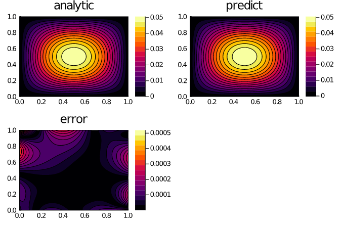
If you use NeuralPDE.jl in your research, please cite this paper:
@article{zubov2021neuralpde,
  title={NeuralPDE: Automating Physics-Informed Neural Networks (PINNs) with Error Approximations},
  author={Zubov, Kirill and McCarthy, Zoe and Ma, Yingbo and Calisto, Francesco and Pagliarino, Valerio and Azeglio, Simone and Bottero, Luca and Luj{\'a}n, Emmanuel and Sulzer, Valentin and Bharambe, Ashutosh and others},
  journal={arXiv preprint arXiv:2107.09443},
  year={2021}
}