By Joe Ganser
Data on superconductors was studied with the goal of predicting the critical temperature at which a material undergoes superconductivity; hence a regession task. The data initially consisted of 168 features and 21,263 rows. The goal was not to predict whether or not a material was superconductive, because all data was on superconductive materials. Another researcher had gotten a root mean squared error (RMSE) of ±9.5kelvin on this data set, and this project's goal was to out perform this metric while comparing model techniques and analyzing features. This study was able to get ±9.4Kelvin RMSE. The data is originally sourced from the superconducting material database. This paper is oriented towards an audience of scientists, and was coded in python 3.6.
- Introduction
- Background info: What is a super conductor?
- Pre-processing the target variable
- Filtering out irrelevant features
- Selecting the right model
- Random Forest: Tuning hyperparameters
- Checking for a good fit
- Feature importance
- Conclusions
- Links to coded notebooks
- Sources
There were several objectives to this project
- Predict the temperature of superconductivity with the highest possible R2 score and lowest possible RMSE
- Compare multiple model techniques and find the one that produces the best metrics
- Identify relevant and irrelevant features
- Ensure model validity
The approach was to first identify the irrelevant features and discard them, followed by putting the remaining features into a bunch of models for wide comparison.
A superconductor is a material that, at a very, very low temperature allows for infinite conductivity (zero electrical resistance). Essentialy this means thats all the electrons/ions will flow on a material without any disturbance what so ever. One of the most interesting things about superconductors is that at their critical temperature they can create magnetic levitation! This is called the Meissner effect. Lexus, the car company, used this phenomenon to create a hoverboard.
The temperature of at which a material becomes superconductive was what I was trying to predict in this analysis. So why is temperature relevant to super conductivity? To understand this, consider a familiar example of something that's the complete opposite.
A toaster works using electrical resistance. In the circuit of a toaster, the electrons are forced to slow down and colide with each other, which in turn causes an accumulation of thermal energy. That thermal energy then raises the temperature, which cooks the toast.
The physics of a super conductor is (sort of) like the opposite of a toaster. Instead of electrons bumnping into each other chaotically (creating heat), the cold causes them all move uniformly. When the temperature is low enough, the uniform motion of the electrons becomes comes very coherent, producing powerful magnetic fields.
There are many materials that can support superconductivity. Each one is a combination of many different elements, and has many intrinsic properties. Thus by creating a table for each super conductor's properties, along with it's critical temperature, a regression analysis can be done.
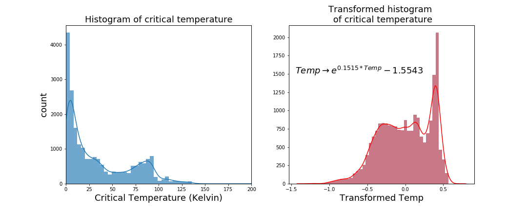
In any regression problem, you want the target variable to be as close to a normal distribution as possible. Sometimes this is possible to do, other times not. In this case I was able to transform the critical temperature to be approximately normal.
Originally the data was very, very positively skewed. After a lot of trial and error, I used an exponential transformation to get the data (approximately) normal.
Unfortunately in the best fit there remained a slight skew. The highest peak wasn't simply an outlier and couldn't be dropped or imputed. Despite this, the results observed at the end were pretty good.Initially the data shape was 21263 rows by 168 features. The head of the original dataframe looked like this;
| number_of_elements | mean_atomic_mass | wtd_mean_atomic_mass | gmean_atomic_mass | wtd_gmean_atomic_mass | entropy_atomic_mass | wtd_entropy_atomic_mass | range_atomic_mass | wtd_range_atomic_mass | std_atomic_mass | wtd_std_atomic_mass | mean_fie | wtd_mean_fie | gmean_fie | wtd_gmean_fie | entropy_fie | wtd_entropy_fie | range_fie | wtd_range_fie | std_fie | wtd_std_fie | mean_atomic_radius | wtd_mean_atomic_radius | gmean_atomic_radius | wtd_gmean_atomic_radius | entropy_atomic_radius | wtd_entropy_atomic_radius | range_atomic_radius | wtd_range_atomic_radius | std_atomic_radius | wtd_std_atomic_radius | mean_Density | wtd_mean_Density | gmean_Density | wtd_gmean_Density | entropy_Density | wtd_entropy_Density | range_Density | wtd_range_Density | std_Density | wtd_std_Density | mean_ElectronAffinity | wtd_mean_ElectronAffinity | gmean_ElectronAffinity | wtd_gmean_ElectronAffinity | entropy_ElectronAffinity | wtd_entropy_ElectronAffinity | range_ElectronAffinity | wtd_range_ElectronAffinity | std_ElectronAffinity | wtd_std_ElectronAffinity | mean_FusionHeat | wtd_mean_FusionHeat | gmean_FusionHeat | wtd_gmean_FusionHeat | entropy_FusionHeat | wtd_entropy_FusionHeat | range_FusionHeat | wtd_range_FusionHeat | std_FusionHeat | wtd_std_FusionHeat | mean_ThermalConductivity | wtd_mean_ThermalConductivity | gmean_ThermalConductivity | wtd_gmean_ThermalConductivity | entropy_ThermalConductivity | wtd_entropy_ThermalConductivity | range_ThermalConductivity | wtd_range_ThermalConductivity | std_ThermalConductivity | wtd_std_ThermalConductivity | mean_Valence | wtd_mean_Valence | gmean_Valence | wtd_gmean_Valence | entropy_Valence | wtd_entropy_Valence | range_Valence | wtd_range_Valence | std_Valence | wtd_std_Valence | critical_temp | H | He | Li | Be | B | C | N | O | F | Ne | Na | Mg | Al | Si | P | S | Cl | Ar | K | Ca | Sc | Ti | V | Cr | Mn | Fe | Co | Ni | Cu | Zn | Ga | Ge | As | Se | Br | Kr | Rb | Sr | Y | Zr | Nb | Mo | Tc | Ru | Rh | Pd | Ag | Cd | In | Sn | Sb | Te | I | Xe | Cs | Ba | La | Ce | Pr | Nd | Pm | Sm | Eu | Gd | Tb | Dy | Ho | Er | Tm | Yb | Lu | Hf | Ta | W | Re | Os | Ir | Pt | Au | Hg | Tl | Pb | Bi | Po | At | Rn |
|---|---|---|---|---|---|---|---|---|---|---|---|---|---|---|---|---|---|---|---|---|---|---|---|---|---|---|---|---|---|---|---|---|---|---|---|---|---|---|---|---|---|---|---|---|---|---|---|---|---|---|---|---|---|---|---|---|---|---|---|---|---|---|---|---|---|---|---|---|---|---|---|---|---|---|---|---|---|---|---|---|---|---|---|---|---|---|---|---|---|---|---|---|---|---|---|---|---|---|---|---|---|---|---|---|---|---|---|---|---|---|---|---|---|---|---|---|---|---|---|---|---|---|---|---|---|---|---|---|---|---|---|---|---|---|---|---|---|---|---|---|---|---|---|---|---|---|---|---|---|---|---|---|---|---|---|---|---|---|---|---|---|---|---|---|---|---|---|
| 4 | 88.9444675 | 57.862692285714296 | 66.36159243157189 | 36.1166119053847 | 1.1817952393305 | 1.06239554519617 | 122.90607 | 31.7949208571429 | 51.968827786103404 | 53.6225345301219 | 775.425 | 1010.26857142857 | 718.1528999521299 | 938.016780052204 | 1.30596703599158 | 0.791487788469155 | 810.6 | 735.9857142857139 | 323.811807806633 | 355.562966713294 | 160.25 | 105.514285714286 | 136.126003095455 | 84.528422716633 | 1.2592439721428899 | 1.2070399870146102 | 205 | 42.914285714285704 | 75.23754049674942 | 69.2355694829807 | 4654.35725 | 2961.5022857142894 | 724.953210852388 | 53.5438109235142 | 1.03312880053102 | 0.814598190091683 | 8958.571 | 1579.58342857143 | 3306.1628967555 | 3572.5966237083794 | 81.8375 | 111.72714285714301 | 60.1231785550982 | 99.4146820543113 | 1.15968659338134 | 0.7873816907632231 | 127.05 | 80.9871428571429 | 51.4337118896741 | 42.55839575195 | 6.9055 | 3.8468571428571403 | 3.4794748493632697 | 1.04098598567486 | 1.08857534188499 | 0.994998193254128 | 12.878 | 1.7445714285714298 | 4.599064116752451 | 4.66691955388659 | 107.75664499999999 | 61.0151885714286 | 7.06248773046785 | 0.62197948704754 | 0.308147989812345 | 0.262848266362233 | 399.97342000000003 | 57.12766857142861 | 168.854243757651 | 138.51716251123 | 2.25 | 2.25714285714286 | 2.2133638394006403 | 2.21978342968743 | 1.36892236074022 | 1.0662210317362 | 1 | 1.08571428571429 | 0.43301270189221897 | 0.43705881545081 | 29.0 | 0.0 | 0 | 0.0 | 0.0 | 0.0 | 0.0 | 0.0 | 4.0 | 0.0 | 0 | 0.0 | 0.0 | 0.0 | 0.0 | 0.0 | 0.0 | 0.0 | 0 | 0.0 | 0.0 | 0.0 | 0.0 | 0.0 | 0.0 | 0.0 | 0.0 | 0.0 | 0.0 | 1.0 | 0.0 | 0.0 | 0.0 | 0.0 | 0.0 | 0.0 | 0 | 0.0 | 0.0 | 0.0 | 0.0 | 0.0 | 0.0 | 0.0 | 0.0 | 0.0 | 0.0 | 0.0 | 0.0 | 0.0 | 0.0 | 0.0 | 0.0 | 0.0 | 0 | 0.0 | 0.2 | 1.8 | 0.0 | 0.0 | 0.0 | 0 | 0.0 | 0.0 | 0.0 | 0.0 | 0.0 | 0.0 | 0.0 | 0.0 | 0.0 | 0.0 | 0.0 | 0.0 | 0.0 | 0.0 | 0.0 | 0.0 | 0.0 | 0.0 | 0.0 | 0.0 | 0.0 | 0.0 | 0 | 0 | 0 |
| 5 | 92.729214 | 58.518416142857106 | 73.13278722250651 | 36.3966020291995 | 1.44930919335685 | 1.05775512271911 | 122.90607 | 36.161939000000004 | 47.094633170313394 | 53.9798696513451 | 766.44 | 1010.61285714286 | 720.605510513725 | 938.745412527433 | 1.5441445432697298 | 0.8070782149387309 | 810.6 | 743.164285714286 | 290.183029138508 | 354.963511171592 | 161.2 | 104.971428571429 | 141.465214777999 | 84.3701669575628 | 1.50832754035259 | 1.2041147982326001 | 205 | 50.571428571428605 | 67.321319060161 | 68.0088169554027 | 5821.4858 | 3021.01657142857 | 1237.09508033858 | 54.0957182556368 | 1.3144421846210501 | 0.9148021770663429 | 10488.571000000002 | 1667.3834285714302 | 3767.4031757706202 | 3632.64918471043 | 90.89 | 112.316428571429 | 69.8333146094209 | 101.166397739874 | 1.42799655342352 | 0.83866646563365 | 127.05 | 81.2078571428572 | 49.438167441765096 | 41.6676207979191 | 7.7844 | 3.7968571428571405 | 4.40379049753476 | 1.0352511158281401 | 1.37497728009085 | 1.07309384625263 | 12.878 | 1.59571428571429 | 4.473362654648071 | 4.60300005985449 | 172.20531599999998 | 61.37233142857139 | 16.0642278788044 | 0.6197346323305469 | 0.847404163195705 | 0.5677061078766371 | 429.97342000000003 | 51.4133828571429 | 198.554600255545 | 139.630922368904 | 2.0 | 2.25714285714286 | 1.8881750225898 | 2.2106794087065498 | 1.55711309805765 | 1.04722136819323 | 2 | 1.12857142857143 | 0.6324555320336761 | 0.468606270481621 | 26.0 | 0.0 | 0 | 0.0 | 0.0 | 0.0 | 0.0 | 0.0 | 4.0 | 0.0 | 0 | 0.0 | 0.0 | 0.0 | 0.0 | 0.0 | 0.0 | 0.0 | 0 | 0.0 | 0.0 | 0.0 | 0.0 | 0.0 | 0.0 | 0.0 | 0.0 | 0.0 | 0.0 | 0.9 | 0.0 | 0.0 | 0.0 | 0.0 | 0.0 | 0.0 | 0 | 0.0 | 0.0 | 0.0 | 0.0 | 0.0 | 0.0 | 0.0 | 0.0 | 0.0 | 0.0 | 0.1 | 0.0 | 0.0 | 0.0 | 0.0 | 0.0 | 0.0 | 0 | 0.0 | 0.1 | 1.9 | 0.0 | 0.0 | 0.0 | 0 | 0.0 | 0.0 | 0.0 | 0.0 | 0.0 | 0.0 | 0.0 | 0.0 | 0.0 | 0.0 | 0.0 | 0.0 | 0.0 | 0.0 | 0.0 | 0.0 | 0.0 | 0.0 | 0.0 | 0.0 | 0.0 | 0.0 | 0 | 0 | 0 |
| 4 | 88.9444675 | 57.885241857142894 | 66.36159243157189 | 36.1225090359592 | 1.1817952393305 | 0.9759804641654979 | 122.90607 | 35.741099 | 51.968827786103404 | 53.65626773209821 | 775.425 | 1010.82 | 718.1528999521299 | 939.009035665864 | 1.30596703599158 | 0.773620193146673 | 810.6 | 743.164285714286 | 323.811807806633 | 354.804182855034 | 160.25 | 104.685714285714 | 136.126003095455 | 84.214573243296 | 1.2592439721428899 | 1.13254686280436 | 205 | 49.31428571428571 | 75.23754049674942 | 67.797712320685 | 4654.35725 | 2999.15942857143 | 724.953210852388 | 53.9740223651659 | 1.03312880053102 | 0.760305152674073 | 8958.571 | 1667.3834285714302 | 3306.1628967555 | 3592.01928133231 | 81.8375 | 112.213571428571 | 60.1231785550982 | 101.082152388012 | 1.15968659338134 | 0.7860067360250121 | 127.05 | 81.2078571428572 | 51.4337118896741 | 41.63987779712121 | 6.9055 | 3.8225714285714303 | 3.4794748493632697 | 1.03743942474191 | 1.08857534188499 | 0.927479442031317 | 12.878 | 1.75714285714286 | 4.599064116752451 | 4.64963546519334 | 107.75664499999999 | 60.94376 | 7.06248773046785 | 0.6190946827042739 | 0.308147989812345 | 0.250477444193951 | 399.97342000000003 | 57.12766857142861 | 168.854243757651 | 138.54061273834998 | 2.25 | 2.27142857142857 | 2.2133638394006403 | 2.23267852196607 | 1.36892236074022 | 1.02917468729772 | 1 | 1.11428571428571 | 0.43301270189221897 | 0.444696640464954 | 19.0 | 0.0 | 0 | 0.0 | 0.0 | 0.0 | 0.0 | 0.0 | 4.0 | 0.0 | 0 | 0.0 | 0.0 | 0.0 | 0.0 | 0.0 | 0.0 | 0.0 | 0 | 0.0 | 0.0 | 0.0 | 0.0 | 0.0 | 0.0 | 0.0 | 0.0 | 0.0 | 0.0 | 1.0 | 0.0 | 0.0 | 0.0 | 0.0 | 0.0 | 0.0 | 0 | 0.0 | 0.0 | 0.0 | 0.0 | 0.0 | 0.0 | 0.0 | 0.0 | 0.0 | 0.0 | 0.0 | 0.0 | 0.0 | 0.0 | 0.0 | 0.0 | 0.0 | 0 | 0.0 | 0.1 | 1.9 | 0.0 | 0.0 | 0.0 | 0 | 0.0 | 0.0 | 0.0 | 0.0 | 0.0 | 0.0 | 0.0 | 0.0 | 0.0 | 0.0 | 0.0 | 0.0 | 0.0 | 0.0 | 0.0 | 0.0 | 0.0 | 0.0 | 0.0 | 0.0 | 0.0 | 0.0 | 0 | 0 | 0 |
| 4 | 88.9444675 | 57.8739670714286 | 66.36159243157189 | 36.1195603503211 | 1.1817952393305 | 1.0222908923957 | 122.90607 | 33.7680099285714 | 51.968827786103404 | 53.63940496787 | 775.425 | 1010.54428571429 | 718.1528999521299 | 938.512776724546 | 1.30596703599158 | 0.7832066603612908 | 810.6 | 739.575 | 323.811807806633 | 355.18388442194396 | 160.25 | 105.1 | 136.126003095455 | 84.371352045645 | 1.2592439721428899 | 1.17303291789271 | 205 | 46.11428571428571 | 75.23754049674942 | 68.52166497852029 | 4654.35725 | 2980.33085714286 | 724.953210852388 | 53.758486291021796 | 1.03312880053102 | 0.7888885322214609 | 8958.571 | 1623.48342857143 | 3306.1628967555 | 3582.3705966440502 | 81.8375 | 111.970357142857 | 60.1231785550982 | 100.24495020209 | 1.15968659338134 | 0.7869004893749151 | 127.05 | 81.0975 | 51.4337118896741 | 42.1023442240235 | 6.9055 | 3.83471428571429 | 3.4794748493632697 | 1.0392111922717702 | 1.08857534188499 | 0.96403104867923 | 12.878 | 1.7445714285714298 | 4.599064116752451 | 4.658301352402599 | 107.75664499999999 | 60.97947428571429 | 7.06248773046785 | 0.6205354084838871 | 0.308147989812345 | 0.257045108326848 | 399.97342000000003 | 57.12766857142861 | 168.854243757651 | 138.528892724768 | 2.25 | 2.26428571428571 | 2.2133638394006403 | 2.2262216392083 | 1.36892236074022 | 1.04883427304761 | 1 | 1.1 | 0.43301270189221897 | 0.440952123830019 | 22.0 | 0.0 | 0 | 0.0 | 0.0 | 0.0 | 0.0 | 0.0 | 4.0 | 0.0 | 0 | 0.0 | 0.0 | 0.0 | 0.0 | 0.0 | 0.0 | 0.0 | 0 | 0.0 | 0.0 | 0.0 | 0.0 | 0.0 | 0.0 | 0.0 | 0.0 | 0.0 | 0.0 | 1.0 | 0.0 | 0.0 | 0.0 | 0.0 | 0.0 | 0.0 | 0 | 0.0 | 0.0 | 0.0 | 0.0 | 0.0 | 0.0 | 0.0 | 0.0 | 0.0 | 0.0 | 0.0 | 0.0 | 0.0 | 0.0 | 0.0 | 0.0 | 0.0 | 0 | 0.0 | 0.15 | 1.85 | 0.0 | 0.0 | 0.0 | 0 | 0.0 | 0.0 | 0.0 | 0.0 | 0.0 | 0.0 | 0.0 | 0.0 | 0.0 | 0.0 | 0.0 | 0.0 | 0.0 | 0.0 | 0.0 | 0.0 | 0.0 | 0.0 | 0.0 | 0.0 | 0.0 | 0.0 | 0 | 0 | 0 |
| 4 | 88.9444675 | 57.840142714285705 | 66.36159243157189 | 36.11071573753821 | 1.1817952393305 | 1.12922373013507 | 122.90607 | 27.8487427142857 | 51.968827786103404 | 53.5887706050743 | 775.425 | 1009.7171428571401 | 718.1528999521299 | 937.025572960086 | 1.30596703599158 | 0.8052296408133571 | 810.6 | 728.8071428571429 | 323.811807806633 | 356.31928137213 | 160.25 | 106.342857142857 | 136.126003095455 | 84.8434418389765 | 1.2592439721428899 | 1.26119371912948 | 205 | 36.514285714285705 | 75.23754049674942 | 70.63444843787241 | 4654.35725 | 2923.8451428571398 | 724.953210852388 | 53.1170285737926 | 1.03312880053102 | 0.859810869291435 | 8958.571 | 1491.78342857143 | 3306.1628967555 | 3552.6686635803203 | 81.8375 | 111.24071428571399 | 60.1231785550982 | 97.7747186271033 | 1.15968659338134 | 0.7873961825201741 | 127.05 | 80.76642857142859 | 51.4337118896741 | 43.4520592088545 | 6.9055 | 3.8711428571428597 | 3.4794748493632697 | 1.04454467078021 | 1.08857534188499 | 1.04496953590973 | 12.878 | 1.7445714285714298 | 4.599064116752451 | 4.6840139510763095 | 107.75664499999999 | 61.0866171428571 | 7.06248773046785 | 0.624877733754845 | 0.308147989812345 | 0.272819938850094 | 399.97342000000003 | 57.12766857142861 | 168.854243757651 | 138.493671473918 | 2.25 | 2.24285714285714 | 2.2133638394006403 | 2.20696281450132 | 1.36892236074022 | 1.0960519179005401 | 1 | 1.05714285714286 | 0.43301270189221897 | 0.42880945770867496 | 23.0 | 0.0 | 0 | 0.0 | 0.0 | 0.0 | 0.0 | 0.0 | 4.0 | 0.0 | 0 | 0.0 | 0.0 | 0.0 | 0.0 | 0.0 | 0.0 | 0.0 | 0 | 0.0 | 0.0 | 0.0 | 0.0 | 0.0 | 0.0 | 0.0 | 0.0 | 0.0 | 0.0 | 1.0 | 0.0 | 0.0 | 0.0 | 0.0 | 0.0 | 0.0 | 0 | 0.0 | 0.0 | 0.0 | 0.0 | 0.0 | 0.0 | 0.0 | 0.0 | 0.0 | 0.0 | 0.0 | 0.0 | 0.0 | 0.0 | 0.0 | 0.0 | 0.0 | 0 | 0.0 | 0.3 | 1.7 | 0.0 | 0.0 | 0.0 | 0 | 0.0 | 0.0 | 0.0 | 0.0 | 0.0 | 0.0 | 0.0 | 0.0 | 0.0 | 0.0 | 0.0 | 0.0 | 0.0 | 0.0 | 0.0 | 0.0 | 0.0 | 0.0 | 0.0 | 0.0 | 0.0 | 0.0 | 0 | 0 | 0 |
Thus, several steps were taken to eliminate the irrelevant features. Specifically;
- Dropping features that varied 5% of less across all rows (using
VarianceThreshold) - Dropping duplicated features (using
.transpose().drop_duplicates(keep='first').transpose()) - Dropping features with a very small correlation with the target variable (less than |+-0.1|)
- Dropping features that were highly correlated with each other (greater than |+-0.8|)
It was concluded that 132 features out of the original 168 had very little relevance.
The data that remained, which would be used for modelling, had 36 features and 21263 rows.
The head of the cleaned dataframe was;
| number_of_elements | mean_atomic_mass | range_atomic_mass | wtd_range_atomic_mass | mean_fie | wtd_mean_fie | wtd_entropy_fie | range_fie | wtd_range_fie | mean_atomic_radius | wtd_range_atomic_radius | mean_Density | range_Density | mean_ElectronAffinity | wtd_mean_ElectronAffinity | range_ElectronAffinity | wtd_range_ElectronAffinity | mean_FusionHeat | range_FusionHeat | mean_ThermalConductivity | wtd_mean_ThermalConductivity | gmean_ThermalConductivity | wtd_entropy_ThermalConductivity | range_ThermalConductivity | range_Valence | wtd_range_Valence | critical_temp | O | S | Ca | Cu | Sr | Y | Ba | Tl | Bi |
|---|---|---|---|---|---|---|---|---|---|---|---|---|---|---|---|---|---|---|---|---|---|---|---|---|---|---|---|---|---|---|---|---|---|---|---|
| 4.0 | 88.9444675 | 122.90607 | 31.7949208571429 | 775.425 | 1010.26857142857 | 0.791487788469155 | 810.6 | 735.9857142857139 | 160.25 | 42.914285714285704 | 4654.35725 | 8958.571 | 81.8375 | 111.72714285714301 | 127.05 | 80.9871428571429 | 6.9055 | 12.878 | 107.75664499999999 | 61.0151885714286 | 7.06248773046785 | 0.262848266362233 | 399.97342000000003 | 1.0 | 1.08571428571429 | 29.0 | 4.0 | 0.0 | 0.0 | 1.0 | 0.0 | 0.0 | 0.2 | 0.0 | 0.0 |
| 5.0 | 92.729214 | 122.90607 | 36.161939000000004 | 766.44 | 1010.61285714286 | 0.8070782149387309 | 810.6 | 743.164285714286 | 161.2 | 50.571428571428605 | 5821.4858 | 10488.571000000002 | 90.89 | 112.316428571429 | 127.05 | 81.2078571428572 | 7.7844 | 12.878 | 172.20531599999998 | 61.37233142857139 | 16.0642278788044 | 0.5677061078766371 | 429.97342000000003 | 2.0 | 1.12857142857143 | 26.0 | 4.0 | 0.0 | 0.0 | 0.9 | 0.0 | 0.0 | 0.1 | 0.0 | 0.0 |
| 4.0 | 88.9444675 | 122.90607 | 35.741099 | 775.425 | 1010.82 | 0.773620193146673 | 810.6 | 743.164285714286 | 160.25 | 49.31428571428571 | 4654.35725 | 8958.571 | 81.8375 | 112.213571428571 | 127.05 | 81.2078571428572 | 6.9055 | 12.878 | 107.75664499999999 | 60.94376 | 7.06248773046785 | 0.250477444193951 | 399.97342000000003 | 1.0 | 1.11428571428571 | 19.0 | 4.0 | 0.0 | 0.0 | 1.0 | 0.0 | 0.0 | 0.1 | 0.0 | 0.0 |
| 4.0 | 88.9444675 | 122.90607 | 33.7680099285714 | 775.425 | 1010.54428571429 | 0.7832066603612908 | 810.6 | 739.575 | 160.25 | 46.11428571428571 | 4654.35725 | 8958.571 | 81.8375 | 111.970357142857 | 127.05 | 81.0975 | 6.9055 | 12.878 | 107.75664499999999 | 60.97947428571429 | 7.06248773046785 | 0.257045108326848 | 399.97342000000003 | 1.0 | 1.1 | 22.0 | 4.0 | 0.0 | 0.0 | 1.0 | 0.0 | 0.0 | 0.15 | 0.0 | 0.0 |
| 4.0 | 88.9444675 | 122.90607 | 27.8487427142857 | 775.425 | 1009.7171428571401 | 0.8052296408133571 | 810.6 | 728.8071428571429 | 160.25 | 36.514285714285705 | 4654.35725 | 8958.571 | 81.8375 | 111.24071428571399 | 127.05 | 80.76642857142859 | 6.9055 | 12.878 | 107.75664499999999 | 61.0866171428571 | 7.06248773046785 | 0.272819938850094 | 399.97342000000003 | 1.0 | 1.05714285714286 | 23.0 | 4.0 | 0.0 | 0.0 | 1.0 | 0.0 | 0.0 | 0.3 | 0.0 | 0.0 |
Seven different types of regression were performed on the data, with the intention of simply estimating the performance of each one without tuning hyperparameters. The metrics of evaluation for each one were the R2 score and the root mean squared error (RMSE). I also measured the time required for each model to fit and predict the data. After all the models and metrics were observed, the best performing one was then selected hyperparameter tuning.
- Ordinary Least Squares
- Ridge Regression
- Lasso Regression
- Elastic Net regression
- Bayesian Ridge
- K-nearest neighbors regression
- Random Forest Regression
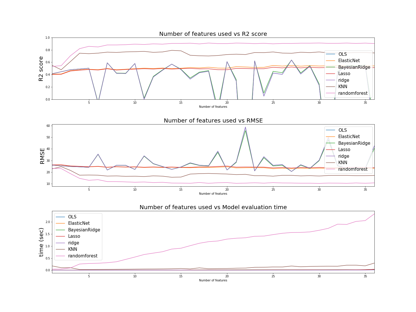
The process of evaluating the models was done by a for loop. At each loop, a sequentially increasing number of features from the data was used on all the models. The order of the features fed into the models was based upon the magnitude of correlation each feature had with the critical_temperature. Hence the first feature used was range_ThermalConductivity which had a correlation of 0.687654, and the last feature was mean_fie which had a correlation of 0.102268. The loop passed through all 36 features. The first iteration had the first feature, the second had the first two features, the third had the first three, and so on. Each model was initially fit without tuning hyperparameters.
In code, the structure was;
#get the correlation of each feature with the target variable
corr = pd.DataFrame(data.corr()['critical_temp'])
#get the absolute value of the correlation
corr['abs'] = np.abs(corr['critical_temp'])
#sort the values by their absolute value, in descending order
corr = corr.sort_values(by='abs',ascending=False)

#loop through the rows of the corr dataframe, getting each feature sequentially
for row in corr.index:
    #add more features iteratively & cumulatively, in order of correlation magnitude
    features = list(corr['index'].loc[:row])
    #use all those features up to that point
    X = df[features]
    X_train, X_test, y_train, y_test = train_test_split(X, y, test_size=0.3, random_state=10)
    #fit/train the model
    model.fit(X_train,y_train)
    #then do RMSE and R2 scoring
See the links to coded notebooks for actual code
At each iteration the seven models were fit on a 70-30 train test split. The R2 and RMSE were then measured.
Graphing the evaluation metrics of each model as a function of the number of features used, we have;
The best performance metrics by each model were *(without tuning hyperparameters)*;| model | RMSE | R2 score | # of features used | time |
|---|---|---|---|---|
| RandomForestRegressor | 10.3001 | 0.9104 | 30 | 1.6523 |
| KNN | 15.5705 | 0.7917 | 14 | 0.0596 |
| BayesianRidge | 20.5437 | 0.6363 | 27 | 0.0167 |
| Ridge | 20.5642 | 0.6356 | 27 | 0.0061 |
| OLS | 20.5645 | 0.6356 | 27 | 0.0123 |
| ElasticNet | 22.9051 | 0.5479 | 27 | 0.0153 |
| Lasso | 23.5355 | 0.5227 | 27 | 0.0145 |
Thus, the best performing model (Random Forest regressor) was then fine tuned with it's hyperparameters.
Because the main goal is to get the most accurate conclusions about superconductors, accuracy, in this context, is more important than efficiency. Hence, despite random forest regressor being the slowest model to fit the data (over 1 second), it was chosen to be the most important because it had the lowest loss function.
The hyperparameter that was tuned was the number of decision trees in the random forest. To do this,I again used a trial and error approach where I cycled through a range of forest sizes. In conjunction, I also tried using different 'max feature' parameters, specifically log2, sqrt and the default.
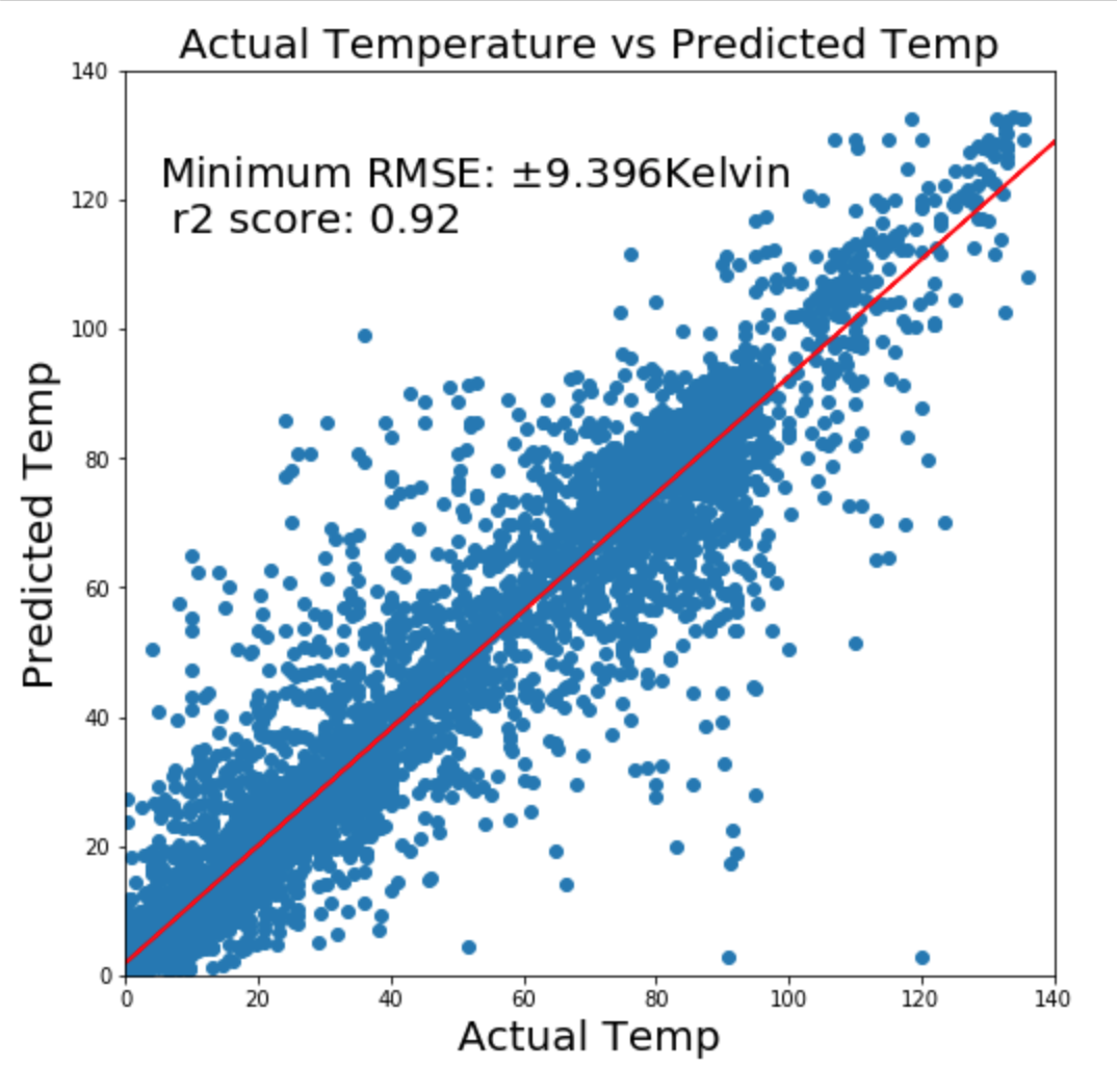
After lots of trial and error, a RMSE of ±9.396Kelvin was found, before tuning it was ±10.3Kelvin.
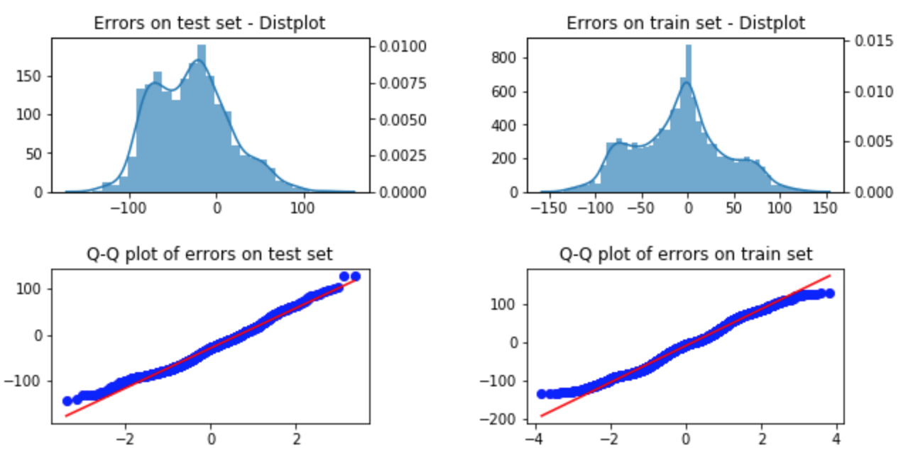
As in any regression analysis, R2 score and RMSE are not the only standards of evaluation. Examining the plot of the predicted values versus actual values is important, as is looking for normality and homoskedascity.
The plot of the predicted temperatures versus actual temperature was
Normality of errors & Homoskedascity
Using seaborn's distplot and probplot functions, I could plot the distribution of errors as well as their Q-Q plots (for both the train sets and the test sets). Approximately normality was observed.
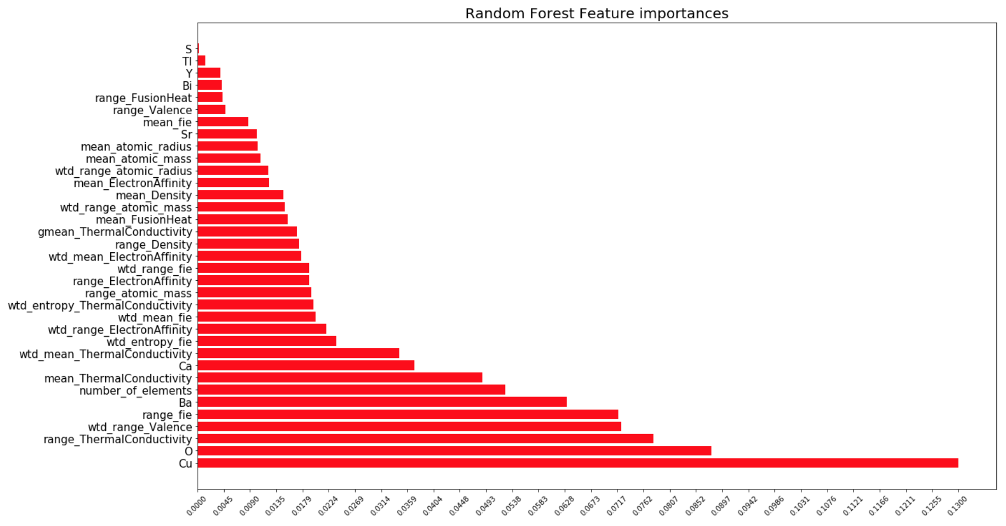
One of the more convenient things about the random forest package is it does feature importance analysis automatically. Here, we can see the relative importances of each measure.
The other researchers that analyzed this data concluded that the important features extracted were ones based on thermal conductivity, atomic radius, valence, electron affinity, and atomic mass. In the graph above we can the same results, with a few extra important features such as the presence of Copper, Oxygen, Barium, the number of elements in the material, et. al. Perhaps it is these few extras I observed that allowed me to get a RMSE of 9.4Kelvin, which is lower than the other research's RMSE of 9.5Kelvin.
- Pre-processing the target variable
- Filtering out irrelevant features
- Selecting the right model
- Tuning Random Forest
- Analyzing prediction errors
- Identifying important features
- A data-driven statistical model for predicting the critical temperature of a superconductor, by Kam Hamidieh
- This was the other research I wanted to compare to.
- UCI Machine learning repository on superconducting data
- The data can be downloaded from here.
- Super conducting material database
- From the National Institute of Material Science; the organization that collected the data

