Tom Bresee, Michael McManus, and Stuart Ong
Written March and April, 2022
For a full review of analysis, please visit the blog on our website.
To use the tool resulting from this analysis please visit HDBestimate.
While there exist numerous studies investigating real estate globally, we were drawn to analyzing Singapore’s resale market for HDB flats which form a natural experiment that enabled us to better isolate and study the effects of location, and location features, on housing values. Across flat types, HDB flats generally have similar sizes, layouts and features, yet we observe significantly varying transaction values. We also observed some of the more expensive resale transactions occurring on older units with shorter remaining leases, running counter to our expectations on leases and depreciation.
Pricing then becomes a key challenge for potential buyers and sellers of HDB resale flats with limited information beyond past transactions and the advice of property agents with potentially skewed incentives (commissions are typically % of transaction value). The goal of our project, HDBestimate, looks to demystify pricing by creating location features and training machine-learning models to predict prices, accounting for these location features. We hypothesize that beyond inherent flat features, location features play a significant role in influencing prices, and we hope to not only provide predictions on price but to also identify how location and different location features actually influence the price of an HDB resale flat.
We explored and examined various factors which included the creation of a large amount of geospatial features used as additional inputs used to accurately predict the flat resale value, and display this information in a clean and highly functional user interface.
All data sources derived from data.gov/sg during the months of March and April in the year 2022
under the terms of the Singapore Open Data Licence version 1.0 .
A full list
of attributed datasets used in this analysis can be found on our
website.
The primary sets of data utilized for the project included Singapore's HDB Resale Flat Prices (Resale transacted prices), and are currently published by the Singapore Housing and Development Board (HDB) and updated on a weekly basis.
Range: Dataset extends from January 1990 through present-day.
-
Baseline dataset consisted of five core data files, covering five time series ranges: 1990-1999, 2000-2012, 2012-2014, 2015-2016, 2017-present day. These files were merged into one consolidated master dataset and imported for analysis.
-
Features from this consolidated set include:
- month (the month/year of the resale transaction)
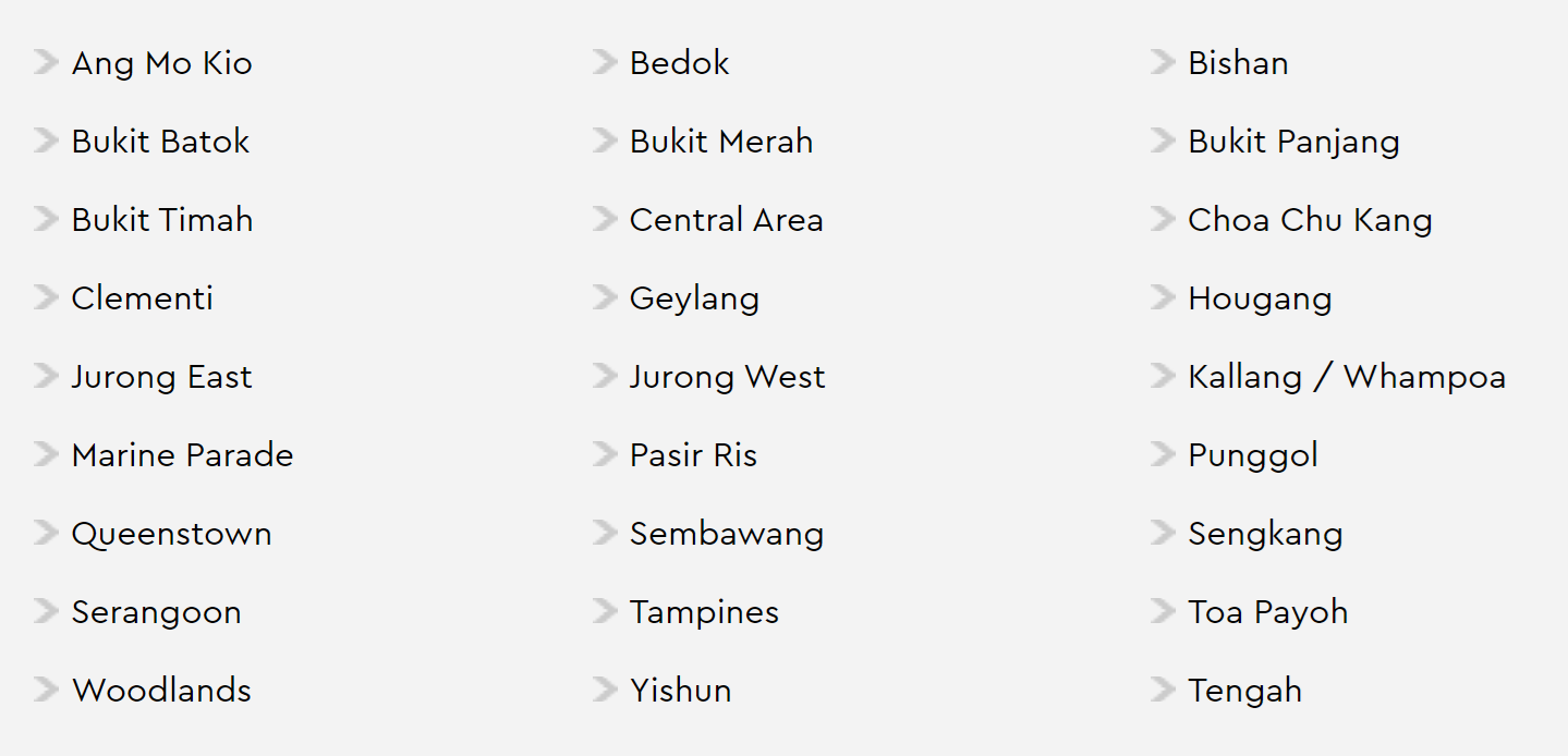
- town (the Singapore town of the actual flat)
- block (the address component of the flat)
- street name (the physical street address)
- flat type (the category of flat including room count)
- floor area (flat's square meter surface floor area)
- flat model (category of flat by model)
- lease commence data (the year the flat was commenced)
- storey range (the range of the flat storey/floor level, e.g. '04 to 06' identifying the flat was in the range between the fourth and sixth storey)
- remaining lease (the remaining years and months of the 99-year lease)
- resale price (price sold for in Singapore dollars, and a major feature of this dataset we will be trying to predict).
-
All towns were detailed and later plotted against various resale pricing data
-
Region breakout shown here
-
Remaining lease: the number of years left before the lease ends; this information is computed as at the resale flat application
-
Resale Price: these should be taken as indicative only as the resale prices agreed between buyers and sellers; these are dependent on many factors which we will explore.
-
Lease left refers to the number of years to the expiry of the 99-year lease; after which, ownership of the HDB will return to the government. This is a very different concept than what is done in the United States.
Total Transaction Observations: 867,677 number of rows, covering 11,747 days
In order to get location for each building in Singapore, we opted to build a scraper (get_postal_codes.ipynb) that used the onemap.sg API. Every building in Singapore is represented by a 6-digit postal code and our scraper queried one million postal codes that ranged from 000000 to 999999, storing the results into a JSON file before finally converting all the results into a dataframe which we upload into our database as the table, sg_buildings_postal.
In addition to the baseline data, we added various location features that we believe would be useful in helping predict flat prices. Location data for each dataset was standardized to the following format:
- SRID: 4326
- Geometries: (Longitude, Latitude)
List of additional location features
After importing the data, we did conventional Exploratory Data Analysis (EDA) to better understand the dataset.
High-level: 867,891 rows of observations encompassing 11 features (month, town, flat_type, block, street_name, storey_range, floor_area_sqm, flat_model, lease_commence_data, resale_price, and remaining_lease). Encompassing 11,747 days of data.
Summarized, this was 27 unique towns, 577 unique street names, 9520 unique addresses, 5 unique regions, 7 unique flat types, 33 flat models, and 25 distinct storey ranges.
Flat Types: The majority of flat types were 4-room (38%), with 3-room (32%) and 5-room (21%) following behind.
4-room flat types were the most transacted flat type in the resale market.
Number of raw rooms: Rooms ranged in count from 1 through 5. 37.6% were 4 room count, 32.4% were 3 room count, and 28.6% were five room count, with 2 and 1 room counts making up less than 1.5%.
Lease commence year spanned from 1966 to 2019.
Floor Space: Square foot in m/s ^ 2 ranged from a minimum of 28, to as large as 307 (a range of 279). Average floor area was 95.7 with a median of 93. The majority of square meter values was in a range from 28 to approximately 160.
Storey Range: The storey ranges continued 25 distinct values, and were somewhat imbalanced, with floors 4-6 (25.2%), floors 7-9 22.8%), floors 1 - 3 (20.3%), and floors 10-12 (19.3%) dominating, and the rest split between the other 21 ranges in a small percentage. Effectively what was determined is that the vast majority of flats did not extend beyond about 20 floors, with outliers going as high as 51 storeys high.
Normalized resale price histogram show a slight right skew, which we kept in mind as we created plots of it versus categorical features.
Plots were created to show the distribution of initial features, the value counts breakout per features, and summary statistics were investigated and plotted as well. We examined features to identify if there were anomalies in the data that were candidates for potential deletion (so as not to skew our model). Average resale price per square-meter versus feature categories showed remarkable insight (these were plotted).
Certain towns appear to have higher value, we can attribute that to locations within the Central Region which is closest to the city center, for instance.
EDA Notebooks:
- One of the strongest correlations was seen between normalized resale price and floor area in sq_m. One would argue that this was to be expected.
- Floor area sq_m and n_rooms
- Floor area sq_m and flat_type (moderate)
- There appeared to be a moderate correlation between resale price and height (storey range). This was confirmed with EDA.
- High correlation, VIF used for analysis
- The top 10 storey_ranges encompassed the vast majority of flats. In addition, there appeared to be a moderate correlation between resale price and height (storey range)
- HDB flat floor area ranged from 28-307 square meters, in a trimodal distribution
- Normalized resale price histogram was right skewed
- One of the strongest correlations was seen between normalize resale price and floor area in sq_m.
- Certain towns appear to have higher value. We can attribute this to locations within the Central Region.
Correlation was done multiple times; on initial data, cleaned data, and final data with location features. The following types of correlation matrices were examined: Spearman, Pearson, Kendall, Cramer, and Phi_k. Some of these compared true numeric values, some could take into consideration categorical, ordinal, and interval variables, in addition to capturing non-linear dependence. Spearman appeared to be able to catch nonlinear monotonic correlations better than Pearsons.
While we had transaction data that ran from 1990, we were cognizant of the fact that there was no time element to our location features. Adding a time element to some location features was not only close to impossible (data not available that far back) but also raised a lot of other questions. For instance, when exactly should we consider count the feature as being in existence there. Some location features, such as restaurants, may not have been in existence for the full duration of our resale transaction data. Using the same example, another possibility is that the restaurant moved during the period between 1990 to present. Another qustion to consider is whether merely was the announcement of a feature sufficient to impact prices prior to the feature actually being built? What about features that move over time? While not the perfect solution, we took the following steps to address these concerns:
- Our features are generally features that are long lasting and not specific (i.e. supermarkets vs a supermarket chain), and typically get replaced with a similar feature
- Shortening our period of analysis to 15 years where most of these features would have already been built/announced. Some features do not typically change over time such as hospitals and police or fire stations
- As a result, we opted to use only 40% of our data starting from 2007 to 2022, with a rough 60-20-20 train/validate/test split by years for our analysis with the training data being the early years and the test data being the later years.
As a result, we opted to use only 40% of our data starting from 2007 to 2022, with a rough 60-20-20 train/validate/test split by years for our analysis with the training data being the early years and the test data being the later years.
Confident that location features add value to the analysis, we next proceeded to explore more complex models that could better describe the data as well as provide some interpretability of the results and predictions. We initially tested Support Vector Machines (SVM) but they not only suffered from long training times but they were not outperforming simpler much better than llinearinear linear regressions. Next we tested baseline untuned decision trees and ensembles (Random Forest/Ada Boost/Gradient Boosting) without hyper-parameter tuning which proved to be much better than linear regressions and SVMs. These methods returned R2 of 91.3% on average on training and 73.3 % on average on the test sets, with random forest and gradient boosting performing the best. We finally opted to go with gradient boosting regressors as we felt that they provided the optimal trade-off between training time and performance and went with the XGBoost package as it allowed us to tune and train models faster with GPU .
As interpretation of coefficients was initially a key focus, we identified that we had strong multicollinearity in our features and in early analysis removed them from our data. However, as we moved deeper into the analysis and on to trees and ensembles our attention turned less to multicollinearity and instead to performance and opted to use as many features as possible. Inadvertently, we ended up including two variables (size and remaining lease years) that were used to derive our target variable which created data leakage. These two features were eventually removed from our final model which we put into production. In our initial analysis, we found that dealing with multicollinearity created a trade-off between model performance and interpretability and we opted to focus on building a model with high predictive power and did not address multicollinearity in our data by removing the features. Ultimately, this had a limited effect on prediction tasks but we need to be more cautious when interpreting features. The final set of features were as follows:
- Conservation Area Map, Eating Establishments, Fire Stations, Hawker Centers, HDB Carpark Information, HDB Property Information
- Hotels, Kindergartens, LTA MRT Station Exit, NParks Parks, Parks, Pre-Schools Location, Private Education Institutions,
- School Directory and Information, SDCP MRT Station Point, Singapore Police Force Establishments, Supermarkets.
Using GridSearchCV, we tuned our XGBoost model using a wide and narrow approach to hyperparameters tuning (first search with a wide range then search around the optimal from the first search).
When optimizing for R2 we found these to be the optimal settings:
max_depth = 3
min_child_weight = 4
gamma = 11
subsample = 0.5
colsample_bytree = 0.5
reg_alpha = 100
reg_lambda = 1
n_estimators = 3000
learning_rate = 0.1
Our model returned an R2 of 90.9% for train and 72.6% for test. We recognize that these are lower than the results of the untrained trees and ensembles but that is because they contain the features that cause the data leak. Including the leak features, we have a test R2 of just under 80%.
# Final Dataset (including location features):  Current Model

# --- R2 Scores ---
Train:       0.962
Validation:  0.897
Test:        0.795

#  --- MSE ---
Train:       11.153
Validation:  40.907
Test:        71.863

# Model Output Results:

--- Test Set ---
Mean Absolute Error: ... 6.078747834396562
Mean Squared Error:..... 67.18
RMSE: .................. 8.196381335337657
Coeff of det (R^2):..... 0.809 (1.4 % better)

--- Val Set ---
Mean Absolute Error: ... 4.498476271962494
Mean Squared Error:..... 38.02
RMSE: .................. 6.166026942280251
Coeff of det (R^2):..... 0.904 (0.7 % better)

--- Train Set ---
Mean Absolute Error: ... 2.339212417385334
Mean Squared Error:..... 10.24
RMSE: .................. 3.200258043072929
Coeff of det (R^2):..... 0.965


# New Model Hyperparameters (XGBoost-based)
    max_depth=7
    min_child_weight=6
    gamma = 10
    subsample=0.75
    colsample_bytree = 0.5
    reg_alpha = 100
    reg_lambda = 1
    n_estimators=800
    learning_rate=0.16
    seed=42
tree_method='hist'Our core data is governed by the Singapore Open Data License, which aims to “promote and enable easy reuse of Public Sector data to create value for the Singapore area community and businesses”. According to the bylaws, the use, access, download, copy, distribution, transmission, modification and adaptation of the datasets, as well as our derived analyses and applications falls under acceptable use according to the license. We followed this bylaw explicitly.
Please Note: The use the datasets does not in a way suggest any official status nor suggest a Singapore agency endorsed us or the use of their datasets. We specifically followed the guidance of the license language and placed a conspicuous notice at the bottom of the website acknowledging the source of the datasets including a link to the most recent version of their posted license.
Note: location data (such as rail station information, locations of taxi stands) are all publicly available. This data was scraped and imported for usage in the modeling.
Some data used in this analysis could provide information with the potential to be misconstrued as a proxy for wealth or social status. Users of the model should understand the intended use of the model and tool is to best estimate the resale value of their HDB Flat and make no causal inference to the "types of people" who may live in these areas. Thoughtful consideration of this concern has been taken throughout the course of this analysis. Further, the Singaporean government has taken steps to mitigate racial conclaves which may otherwise occur by mandating the Ethnic Integration Policy. This integration policy helps to "... ensure a better racial mix in HDB estates, the government established ethnic quotas for HDB neighbourhoods and blocks. The permissible proportion of flats in each neighbourhood for Malays was 22 percent while the permissible proportion of flats in each block was 25 percent. For Chinese, the permissible proportions were 84 percent and 87 percent respectively, and for Indians and other minority groups, the figures were reduced to 10 percent and 13 percent respectively" [1]. While we are confident this policy aids in reducing the perpetuation of biases toward a particular area over another while also realizing it is still possible as the model provided predicts price based on location and in time series. Some biases may be further embedded in Singaporean culture as a result of our analysis and tool.
Modified Distance - Potentially adding a modification of the straight-line geo-spatial distance features in ‘Manhattan’ form (i.e. taxi-cab / city-block geometry). Singapore is a very walkable city, and distances from the HDB flat to nearby feature locations (such as hospitals, etc) many times are only possible via sidewalk or city streets. We also have examined adding potentially in the future a feature of the total travel time (whether walking or driving) to go from the flat to the specific destination location.
Crime Data - Overlaying another set of features associated with historical crime (similar to NY city’s statistics) is an option. Although crime is extremely low in Singapore, it may be interesting to see if this is a factor in resale pricing values.
PLH (Prime Location Housing) - Scenarios where there are no HDBs there currently (and this is direct from HDB, not a resale transaction). PLH is a new scheme of housing that was recently launched which includes more restrictions when it comes to resale. The concept would be that one could say that a resale could potentially fetch a certain dollar amount based on the machine learning model, allowing a mapping from HDB to appreciation of another set amount. This new housing model for public flats in prime areas includes owners of BTO flats in those areas facing a 10-year minimum occupation period; these flats will be priced with additional subsidies; those who sell their BTO units will have to pay back HDB a percentage of the resale price. The resale buyer criteria for these units will be tighter than for typical resale units.
Unsupervised Clustering - Deeper dive into clustering
Interactivity - Plan to investigate adding more features to the front-end application, including additional drop-down menus
Michael - Data gathering, cleaning, and pipelining into the database. Initial database creation. Webapp development and hosting.
Stuart - Data gathering, cleaning, and pipelining into the database. Second/current database creation. XGBoost Model creation and validation. Blog.
Tom - Data analysis and creation of baseline Random Forest Regression model. Blog.