Principal component analysis or Karhunen Loev transformation is a linear transformation via an orthonormal matrix. It allows us to catch the "essence" of a given data set and thus it can be uesd in various ways:
- Dimensionality reduction - often used in image analysis and classification tasks
- Linear decorrelation of data
- Lossy compression
- Data modeling
- ...
PCA is a global subspace method that calculates

x is an input vector, U is a set of basis vectors obtained by PCA and a is a vector in the feature space representing the input vector. It allows to represent high dimensional data such as images with a small set of parameters. PCA thereby tries to seek for a linear projection such that the variability of the input data can be described using only a small number of basis vectors.
PCA is lookig for a set of basis vectors that minimize the reconstruction error in a least squares sense:
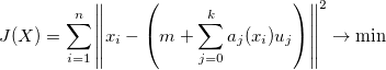
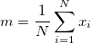
where m is the input data sample mean.
and aj(xi) is the projection of the input data onto U
Solving the minimization problem of J(X) is equivalent to solving the Eigenvalueproblem of the covariance matrix.
This leads to the efficient implementation using singular value decomposition:
If the a matrix X is a set of mean normalized random vectors the covariance matrix C can be achieved from the product X*X'. Since for each matrix A there exist U, S and V so that A = USV' and A' = V*S'*U', where [U,S,V] = svd(A), the covariance matrix can be represented as C = USS'*U'. So one sees that C and A have a intentical set of orthonormal eigenvectors and that the eigenvalues of C are the squared eigenvalues of A.
As a handy property the Eigenvalues scale correlates to the "energy" that the corresponding Eigenvector covers in the underlying data. That means that Eigenvectors with small Eigenvalues can be discarded but the reconstructed item is still close to original input in a least squares sense. That property can be used for data modeling, dimensionality reduction and compression algorithms.
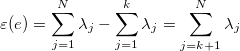
The more formal way is: The variance in the direction of ui is equal to the i-th eigenvalue _lambdai. When using all eigenvectors the input data can be reconstructed without any reconstruction error. By choosing only the k largest eigenvalues with the corresponding eigenvectors the expected mean square error epsilon is given by
The PCA class also offers a way to calculate the PCA in a wheighted manner - meaning that single examples are more important than others and thus have more influence on the covariance matrix.
The algorithm is basically the same with the following differences:
- We have a weight for each example - all weights have to sum up to one
- The mean value is a weighted mean
- Each input example is scaled by it's associated weight.
PCA as is - as every standard least squares algorithm - not very robust agains values that are out of the normal, expected range. In fact a single outlier - e.g. a cluttered pixel or even worse a whole area - can destroy the projection and reconstruction in the PCA algorithm. To circumvent this one can first find these outliers (or even regions) and not use them in the projection step. This is possible since in most cases the size of an example is mostly most larger than the size of input examples thus we have an overdetermined equation system. Normally that is solved by multiplying the input examples with the Eigenvectors so we get a least square optimal solution but of course one does not need to use all of them. By identifying outlying pixels and removing these from the equation we have a robust but still least square solution of the problem. The outlying elements are identified in an iterative manner - here all elements are thrown away where the reconstruction error is higher than a certain criteria.
An even faster method is described in "Fast Robust PCA" by Markus Storer, Peter M. Roth, Martin Urschler and Horst Bischof which is actually the method used here and includes multiple sub sub spaces that use different random subssets of the original sub space. By checking the outliers there we achieve a faster determination of them. Please refere to the orignal paper for more details.
The incremental version of PCA is based on the algorithms described in: "Robust Subspace Approaches to Visual Learning and Recognition" by Danijel Skocaj whereas the incremental algorithm also takes example weighting into account. The algorithm basically has an upper limit in the number of eigenvectors that are created so we take example by example - update the Eigenvectors and sample mean by performing PCA again and after a rotation operation throw away the Eigenvector with the lowest Eigenvalue.
The same algorithm is also implemented for spatial weights (aka per example feature weights) as well as the fast robust version.
Check out the file "TestPCA.pas" it contains various examples for applying all kind of PCA options on either small matrices or more interstingly on images.
Simple PCA on images with reconstruction:
procedure TTestPCA.TestPCAImages;
var Examples : TDoubleMatrix;
    img : TDoubleMatrix;
    feature : TDoubleMatrix;
    w, h : integer;
    i : integer;
begin
     Examples := LoadImages(w, h);

     // ############################################
     // #### Calculate PCA on images
     with TMatrixPCA.Create([pcaEigVals, pcaMeanNormalizedData, pcaTransposedEigVec]) do
     try
        // main function: Takes a matrix with width=num examples and height=example feature vec
        // and applies PCA on it. The number of preserved Eigenvectors is calculated such
        // that 95% of the Eigenvalue energy is preserved. With an integer value 1 <= val <= width
        // one can define the maximum number of Eigenvectors to keep
        Check(PCA(Examples, 0.95, True) = True, 'Error in PCA');
        // create a few examples along the first mode
        feature := TDoubleMatrix.Create(1, NumModes);
        try
           for i in [0, 1, 2, 3, 4 ] do
           begin
                feature[0, 0] := (i - 2)*sqrt(EigVals[0,0]);
                img := Reconstruct(feature);
                try
                   ImageFromMatrix(img, w, h, Format('%s\bmp1_%d.bmp', [ExtractFilePath(ParamStr(0)), i - 2]));
                finally
                       img.Free;
                end;
           end;
        finally
               feature.Free;
        end;
     finally
            Free;
     end;

     FreeAndNil(examples);
end;
Calculating an incremental PCA on the same set of images.
procedure TTestPCA.TestPCAIncremental;
var Examples : TDoubleMatrix;
    img : TDoubleMatrix;
    feature : TDoubleMatrix;
    w, h : integer;
    i : integer;
begin
     Examples := LoadImages(w, h);

     // ############################################
     // #### Calculate PCA on images
     with TIncrementalPCA.Create([pcaEigVals]) do
     try
	// after we have reached 20 Eigenvectors we start to keep that number constant
        NumEigenvectorsToKeep := 20;

        // ############################################
        // #### Feed the examples
        for i := 0 to Examples.Width - 1 do
        begin
             Examples.SetSubMatrix(i, 0, 1, Examples.Height);
             Check(UpdateEigenspace(Examples), 'Error updating eigenspace');
        end;

        // ############################################
        // #### create a few examples along the first mode
        feature := TDoubleMatrix.Create(1, NumModes);
        try
           for i in [0, 1, 2, 3, 4 ] do
           begin
                feature[0, 0] := (i - 2)*sqrt(EigVals[0,0])/3;
                img := Reconstruct(feature);
                try
                   ImageFromMatrix(img, w, h, Format('%s\bmp_inc_%d.bmp', [ExtractFilePath(ParamStr(0)), i - 2]));
                finally
                       img.Free;
                end;
           end;
        finally
               feature.Free;
        end;
     finally
            Free;
     end;

     FreeAndNil(examples);
end;
An example to use the fast robust algorithm:
procedure TTestPCA.TestFastRobustPCA;
var Examples : TDoubleMatrix;
    img : TDoubleMatrix;
    feature : TDoubleMatrix;
    w, h : integer;
    i : integer;
  //  start : Cardinal;
  //  stop : Cardinal;
    x : integer;
    props : TFastRobustPCAProps;
begin
     Examples := LoadImages(w, h);

     // ############################################
     // #### Calculate PCA on images
     props.NumSubSubSpaces := 100;
     props.SubSpaceSizes := 0.003;          // 0.3% of the sub space
     props.Start := 50;                     // num Eigenvectors*Start random sampled elements used as initialized pixel set
     props.stop := 20;                      // num Eigenvectors*Stop elements used as maximum minimal pixel set
     props.ReductionFactor := 0.75;
     props.SubSpaceCutEPS := 0;             // no sub sub space reduction

     with TFastRobustPCA.Create([pcaTransposedEigVec]) do
     try
        SetProperties(props);
        Check(PCA(Examples, 0.8, True) = True, 'Error in PCA');

        // create 50% random occlusion
        for i := 0 to 5 do
        begin
             for x := 0 to Round(0.5*Examples.Height) do
                 Examples[i, random(Examples.Height - 1)] := 255;
        end;

        // create a few examples along the first mode
        for i := 0 to 5 do
        begin
             Examples.SetSubMatrix(i, 0, 1, Examples.Height);
             feature := ProjectToFeatureSpace(Examples);
             try
                img := Reconstruct(feature);
                try
                   ImageFromMatrix(img, w, h, Format('%s\bmpr_%d.bmp', [ExtractFilePath(ParamStr(0)), i - 2]));
                finally
                       img.Free;
                end;
             finally
                    feature.Free;
             end;

             // ############################################
             // #### For comparison -> project to feature space in a non robust way
             feature := ProjectToFeatureSpaceNonRobust(Examples);
             try
                img := Reconstruct(feature);
                try
                   ImageFromMatrix(img, w, h, Format('%s\bmpnr_%d.bmp', [ExtractFilePath(ParamStr(0)), i - 2]));
                finally
                       img.Free;
                end;
             finally
                    feature.Free;
             end;
        end;
     finally
            Free;
     end;

     FreeAndNil(examples);
end;