Selection of the best model for the pricing of the houses located in wide parts of Bengaluru .
- https://housing.com/in/buy/bangalore/house-bangalore
- https://www.99acres.com/independent-house-in-bangalore-ffid
- https://www.magicbricks.com/independent-house-for-sale-in-bangalore-pppfs
- https://www.commonfloor.com/bangalore-property/for-sale/independent-house-ht
- Linear Regression
- Support Vector Machine
- Random Forest Regressor
- XGBoost
- https://www.jigsawacademy.com/blogs/data-science/types-of-regression-analysis/
- https://www.upgrad.com/blog/types-of-regression-models-in-machine-learning/
- https://www.analyticsvidhya.com/blog/2022/01/different-types-of-regression-models/
- XGboost https://scikit-learn.org/stable/modules/generated/sklearn.ensemble.GradientBoostingClassifier.html
to predict the housing rates of Bangalore city and to understand the best model by taking both the accurace and root mean squared error . The priamry goal is to find the best model and know the best regressor in the model .The algorithms that are used are Linear Regression, Support Vector Machine , Random Forest classifier and one boosting algorithm called as the XGboost.
ohe_data_reduce_cat_class.csvfor the databangalore_data_specifics.txtcollection of the datasetv2-ML Model-bangalore_house_price_prediction.ipynbnotebook and code
imports
import numpy as np
import pandas as pd
import matplotlib.pyplot as plt
import seaborn as sns
from sklearn.model_selection import train_test_split
from sklearn.preprocessing import StandardScaler
from sklearn.linear_model import LinearRegression
from sklearn.linear_model import Lasso
from sklearn.linear_model import Ridge
from sklearn.metrics import mean_squared_error
from sklearn.svm import SVR
from sklearn.ensemble import RandomForestRegressor
import xgboost
from sklearn.model_selection import GridSearchCV
from xgboost.sklearn import XGBRegressor
import joblib
The shape of the dataset if we type df.shape is (7120, 108) , the dataset contains upt0 7000 records and aroound 108 columns . further we drop the first column which has and unnecessary index by df = df.drop(['Unnamed: 0'], axis=1) .
We then split the dataset into x and y and we keep price as the label column, i.e the price column will be used to predict the price of the house depending on the area and then locality.
as you can see the outcomes of the price column we see that the outtcomes are continious in the nature and therefore we need regression alogorithms .
	bath	balcony	price	total_sqft_int	bhk	price_per_sqft	area_typeSuper built-up Area	area_typeBuilt-up Area	area_typePlot Area	availability_Ready To Move	location_Whitefield	location_Sarjapur Road	location_Electronic City	location_Raja Rajeshwari Nagar	location_Marathahalli	location_Haralur Road	location_Hennur Road	location_Bannerghatta Road	location_Uttarahalli	location_Thanisandra	location_Electronic City Phase II	location_Hebbal	location_Yelahanka	location_7th Phase JP Nagar	location_Kanakpura Road	location_KR Puram	location_Sarjapur	location_Rajaji Nagar	location_Bellandur	location_Kasavanhalli	location_Begur Road	location_Kothanur	location_Banashankari	location_Hormavu	location_Harlur	location_Akshaya Nagar	location_Jakkur	location_Electronics City Phase 1	location_Varthur	location_HSR Layout	location_Chandapura	location_Ramamurthy Nagar	location_Hennur	location_Kundalahalli	location_Ramagondanahalli	location_Kaggadasapura	location_Koramangala	location_Hulimavu	location_Budigere	location_Hoodi	location_Malleshwaram	location_JP Nagar	location_Hegde Nagar	location_Yeshwanthpur	location_8th Phase JP Nagar	location_Gottigere	location_Channasandra	location_Bisuvanahalli	location_Vittasandra	location_Indira Nagar	location_Brookefield	location_Vijayanagar	location_Old Airport Road	location_Sahakara Nagar	location_Hosa Road	location_Kengeri	location_Bommasandra	location_Green Glen Layout	location_Balagere	location_Old Madras Road	location_Kudlu Gate	location_Panathur	location_Rachenahalli	location_Yelahanka New Town	location_Jigani	location_Kadugodi	location_Talaghattapura	location_Thigalarapalya	location_Mysore Road	location_Ambedkar Nagar	location_Frazer Town	location_Dodda Nekkundi	location_Attibele	location_Kanakapura	location_Devanahalli	location_Nagarbhavi	location_TC Palaya	location_Lakshminarayana Pura	location_5th Phase JP Nagar	location_Anekal	location_Ananth Nagar	location_Jalahalli	location_CV Raman Nagar	location_Kengeri Satellite Town	location_Kudlu	location_Bhoganhalli	location_Doddathoguru	location_Subramanyapura	location_Kalena Agrahara	location_Horamavu Agara	location_Hosur Road	location_Vidyaranyapura	location_Hebbal Kempapura	location_BTM 2nd Stage	location_Mahadevpura	location_Horamavu Banaswadi	location_Domlur	location_Tumkur Road
0	3.0	2.0	150.0	1672.0	3	8971.291866	1	0	0	1	0	0	0	0	0	0	0	0	0	0	0	0	0	0	0	0	0	0	0	0	0	0	0	0	0	0	0	0	0	0	0	0	0	0	0	0	0	0	0	0	0	0	0	0	0	0	0	0	0	0	0	0	0	0	0	0	0	0	0	0	0	0	0	0	0	0	0	0	0	0	0	0	0	0	0	0	0	0	0	0	0	0	0	0	0	0	0	0	0	0	0	0	0	0	0	0	0	0
1	3.0	3.0	149.0	1750.0	3	8514.285714	0	1	0	1	0	0	0	0	0	0	0	0	0	0	0	0	0	0	0	0	0	0	0	0	0	0	0	0	0	0	0	0	0	0	0	0	0	0	0	0	0	0	0	0	0	0	0	0	0	0	0	0	0	0	0	0	0	0	0	0	0	0	0	0	0	0	0	0	0	0	0	0	0	0	0	0	0	0	0	0	0	0	0	0	0	0	0	0	0	0	0	0	0	0	0	0	0	0	0	0	0	0
2	3.0	2.0	150.0	1750.0	3	8571.428571	1	0	0	1	0	0	0	0	0	0	0	0	0	0	0	0	0	0	0	0	0	0	0	0	0	0	0	0	0	0	0	0	0	0	0	0	0	0	0	0	0	0	0	0	0	0	0	0	0	0	0	0	0	0	0	0	0	0	0	0	0	0	0	0	0	0	0	0	0	0	0	0	0	0	0	0	0	0	0	0	0	0	0	0	0	0	0	0	0	0	0	0	0	0	0	0	0	0	0	0	0	0
3	2.0	2.0	40.0	1250.0	2	3200.000000	1	0	0	1	0	0	0	0	0	0	0	0	0	0	0	0	0	0	0	0	0	0	0	0	0	0	0	0	0	0	0	0	0	0	0	0	0	0	0	0	0	0	0	0	0	0	0	0	0	0	0	0	0	0	0	0	0	0	0	0	0	0	0	0	0	0	0	0	0	0	0	0	0	0	0	0	0	0	0	0	0	0	0	0	0	0	0	0	0	0	0	0	0	0	0	0	0	0	0	0	0	0
4	2.0	2.0	83.0	1200.0	2	6916.666667	0	0	1	1	0	0	0	0	0	0	0	0	0
you can see the dataframe above and this is the operation done by df.head(5). A careful observation of the table will show that the housing depends on the location which corresponds to different distances inside the city
let us take an example here
bath	balcony	price	total_sqft_int	bhk	price_per_sqft	area_typeSuper built-up Area	area_typeBuilt-up Area	area_typePlot Area	availability_Ready To Move	location_Whitefield	location_Sarjapur Road	location_Electronic City	location_Raja Rajeshwari Nagar	location_Marathahalli	location_Haralur Road	location_Hennur Road	location_Bannerghatta Road	location_Uttarahalli	location_Thanisandra	location_Electronic City Phase II	location_Hebbal	location_Yelahanka	location_7th Phase JP Nagar	location_Kanakpura Road	location_KR Puram	location_Sarjapur	location_Rajaji Nagar	location_Bellandur	location_Kasavanhalli	location_Begur Road	location_Kothanur	location_Banashankari	location_Hormavu	location_Harlur	location_Akshaya Nagar	location_Jakkur	location_Electronics City Phase 1	location_Varthur	location_HSR Layout	location_Chandapura	location_Ramamurthy Nagar	location_Hennur	location_Kundalahalli	location_Ramagondanahalli	location_Kaggadasapura	location_Koramangala	location_Hulimavu	location_Budigere	location_Hoodi	location_Malleshwaram	location_JP Nagar	location_Hegde Nagar	location_Yeshwanthpur	location_8th Phase JP Nagar	location_Gottigere	location_Channasandra	location_Bisuvanahalli	location_Vittasandra	location_Indira Nagar	location_Brookefield	location_Vijayanagar	location_Old Airport Road	location_Sahakara Nagar	location_Hosa Road	location_Kengeri	location_Bommasandra	location_Green Glen Layout	location_Balagere	location_Old Madras Road	location_Kudlu Gate	location_Panathur	location_Rachenahalli	location_Yelahanka New Town	location_Jigani	location_Kadugodi	location_Talaghattapura	location_Thigalarapalya	location_Mysore Road	location_Ambedkar Nagar	location_Frazer Town	location_Dodda Nekkundi	location_Attibele	location_Kanakapura	location_Devanahalli	location_Nagarbhavi	location_TC Palaya	location_Lakshminarayana Pura	location_5th Phase JP Nagar	location_Anekal	location_Ananth Nagar	location_Jalahalli	location_CV Raman Nagar	location_Kengeri Satellite Town	location_Kudlu	location_Bhoganhalli	location_Doddathoguru	location_Subramanyapura	location_Kalena Agrahara	location_Horamavu Agara	location_Hosur Road	location_Vidyaranyapura	location_Hebbal Kempapura	location_BTM 2nd Stage	location_Mahadevpura	location_Horamavu Banaswadi	location_Domlur	location_Tumkur Road
7117	2.0	1.0	48.0	880.0	2	5454.545455	0	0	1	1	0	0	0	0	0	0	0	0	0	0	0	0	0	0	0	0	0	0	0	0	0	0	0	0	0	0	0	0	0	0	0	0	0	0	0	0	0	0	0	0	0	0	0	0	0	0
In the table we see that we have 0 and 1 in particular cells in the table , area_typePlot Area and vailability_Ready To Move are filled with 1 in the cell .
1 denotes yes, 0 denotes no
we can see that the price is correleated with the topgraphy and geography of the location and tus it makes sense for the prices to get effected . This is the primary reason we are building various machine learning model to identify the best model for predicting the price of the house based on the location .
X = df.drop("price", axis=1)
y = df['price']
print('Shape of X = ', X.shape)
print('Shape of y = ', y.shape)
X_train, X_test, y_train, y_test = train_test_split(X, y, test_size = 0.2, random_state = 51)
print('Shape of X_train = ', X_train.shape)
print('Shape of y_train = ', y_train.shape)
print('Shape of X_test = ', X_test.shape)
print('Shape of y_test = ', y_test.shape)
we have kept 20% of the data for testing purposes .
after this step it is important to standardize the feature column. Standardization of a dataset is a common requirement for many machine learning estimators: they might behave badly if the individual features do not more or less look like standard normally distributed data (e.g. Gaussian with 0 mean and unit variance).
before we go ahead , lets discuss the lasso,ridge and rmse
Lasso regression stands for Least Absolute Shrinkage and Selection Operator. It adds penalty term to the cost function. This term is the absolute sum of the coefficients. As the value of coefficients increases from 0 this term penalizes, cause model, to decrease the value of coefficients in order to reduce loss. The difference between ridge and lasso regression is that it tends to make coefficients to absolute zero as compared to Ridge which never sets the value of coefficient to absolute zero.
In Ridge regression, we add a penalty term which is equal to the square of the coefficient. The L2 term is equal to the square of the magnitude of the coefficients. We also add a coefficient \lambda to control that penalty term. In this case if \lambda is zero then the equation is the basic OLS else if \lambda , > , 0 then it will add a constraint to the coefficient. As we increase the value of \lambda this constraint causes the value of the coefficient to tend towards zero. This leads to both low variance (as some coefficient leads to negligible effect on prediction) and low bias (minimization of coefficient reduce the dependency of prediction on a particular variable).
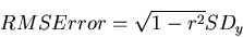
Root Mean Square Error (RMSE) is the standard deviation of the residuals (prediction errors). Residuals are a measure of how far from the regression line data points are; RMSE is a measure of how spread out these residuals are. In other words, it tells you how concentrated the data is around the line of best fit. Root mean square error is commonly used in climatology, forecasting, and regression analysis to verify experimental results.
lr = LinearRegression()
lr_lasso = Lasso()
lr_ridge = Ridge()
lr.fit(X_train, y_train)
lr_score = lr.score(X_test, y_test) # with all num var 0.7842744111909903
lr_rmse = rmse(y_test, lr.predict(X_test))
lr_score, lr_rmse
now when we fit our data to both simple Linear regression and regularized Lasso (l1) we see that the score comes out to be 79% accurate whereas the rmse score comes out to be 64.89%
you can see in the noteboook for the usage of lasso and ridge score too. The lr_lasso score is around 80% and lr_lasso_rmse score is around 62.8%
svr = SVR()
svr.fit(X_train,y_train)
svr_score=svr.score(X_test,y_test) # with 0.2630802200711362
svr_rmse = rmse(y_test, svr.predict(X_test))
svr_score, svr_rmse
we have imported the svr regressor for this regression problem from SVM . The svr score is around 77% and the svr_rmse value is around 64% .
rfr = RandomForestRegressor()
rfr.fit(X_train,y_train)
rfr_score=rfr.score(X_test,y_test) # with 0.8863376025408044
rfr_rmse = rmse(y_test, rfr.predict(X_test))
rfr_score, rfr_rmse
if we were evaluating all the models we cannot ignore the ensembling techniques that provides us the mean or the avearge of the data inside the regression. The averaging makes a Random Forest better than a single Decision Tree hence improves its accuracy and reduces overfitting. A prediction from the Random Forest Regressor is an average of the predictions produced by the trees in the forest.
the normal score is 88% and the rmse is 47% , this definetely overfitting of the data , we have not done cost complexity pruning here because we are evaluating the algorithms based without Hyper parameter tuning with the exception of xgboost.
xgb_reg = xgboost.XGBRegressor()
xgb_reg.fit(X_train,y_train)
xgb_reg_score=xgb_reg.score(X_test,y_test) # with 0.8838865742273464
xgb_reg_rmse = rmse(y_test, xgb_reg.predict(X_test))
xgb_reg_score, xgb_reg_rmse
normal score is 87% and 45% .
                    Model     Score        RMSE
0       Linear Regression  0.790384   64.898435
1                   Lasso  0.803637   62.813243
2  Support Vector Machine  0.206380  126.278064
3           Random Forest  0.889623   47.093442
4                 XGBoost  0.875939   49.927407
till now we have splitted the data in one fold , let us try some cross-validation to get different scores and more model accuracy . But before cross validation and including different folds we have to hyper parameterize the xgboost model for better accuracy and higher score as promised . We then proceed to cross validate random-forest-regressor and Xgboost
- for official documentation of the xgboost parameters - https://xgboost.readthedocs.io/en/stable/parameter.html
- for more knowledge on xgboost tree methods - https://xgboost.readthedocs.io/en/stable/treemethod.html
xgb_tune2 =  XGBRegressor(base_score=0.5, booster='gbtree', colsample_bylevel=1,
             colsample_bynode=0.9, colsample_bytree=1, gamma=0,
             importance_type='gain', learning_rate=0.05, max_delta_step=0,
             max_depth=4, min_child_weight=5, missing=None, n_estimators=100,
             n_jobs=1, nthread=None, objective='reg:linear', random_state=0,
             reg_alpha=0, reg_lambda=1, scale_pos_weight=1, seed=None,
             silent=None, subsample=1, verbosity=1)
xgb_tune2.fit(X_train,y_train) # 0.9412851220926807
xgb_tune2.score(X_test,y_test)
results after hyper-parameter-tuning of Xgboost
- score
88% - rmse
48%
cvs_rfr2 = cross_val_score(RandomForestRegressor(), X_train,y_train, cv = 10)
cvs_rfr2, cvs_rfr2.mean()  #this is for the random regressor


cvs = cross_val_score(xgb_tune2, X_train,y_train, cv = 5)
cvs, cvs.mean()  #this is for the tuned XGboost regressor
outputs in array
(array([0.99494408, 0.96682912, 0.99720454, 0.96433211, 0.96151867,
        0.94774651, 0.94212832, 0.91069009, 0.99610078, 0.98860838]),
 0.9670102612461828)  random forest (10 fold cv)

 (array([0.97924577, 0.98376376, 0.97530216, 0.90127522, 0.96273069]),
 0.9604635172361338) tuned XGboost (5fold-cv)
random forest array mean
from the table and from the tuned xgboost result we now compare the following
                    Model     Score        RMSE
0       Linear Regression  0.790384   64.898435
1                   Lasso  0.803637   62.813243
2  Support Vector Machine  0.206380  126.278064
3           Random Forest  0.889623   47.093442
4                 XGBoost  0.875939   49.927407
5           tuned XGboost   0.88756   48.566634
after properly analysing the results along with the accuaracies and rms errors of the same , we can see that the Linear regression having a score of almsot 80& with rmse score of 65% , th difference is relatively low wehen compared to the other algorithms of which you can see the maximum difference is between the Random-forest algorithm .Although we hace properly tuned XGboost , we can see that the results far have not been improved and it is just a small fraction boost in the results .
Thus we can say that the linear regression is a better algorithm to use in this data as compared to others .
we have also predicted some of the values using both XGboost and Random forest , below is the examplary code snippet
# this method helps in getting the predicted value of house by providing features value
def predict_house_price(model,bath,balcony,total_sqft_int,bhk,price_per_sqft,area_type,availability,location):

  x =np.zeros(len(X.columns)) # create zero numpy array, len = 107 as input value for model

  # adding feature's value according to their column index
  x[0]=bath
  x[1]=balcony
  x[2]=total_sqft_int
  x[3]=bhk
  x[4]=price_per_sqft

  if "availability"=="Ready To Move":
    x[8]=1

  if 'area_type'+area_type in X.columns:
    area_type_index = np.where(X.columns=="area_type"+area_type)[0][0]
    x[area_type_index] =1

    #print(area_type_index)

  if 'location_'+location in X.columns:
    loc_index = np.where(X.columns=="location_"+location)[0][0]
    x[loc_index] =1

    #print(loc_index)

  #print(x)

  # feature scaling
  x = sc.transform([x])[0] # give 2d np array for feature scaling and get 1d scaled np array
  #print(x)

  return model.predict([x])[0] # return the predicted value by train XGBoost model


  predict_house_price(model=xgb_tune2, bath=3,balcony=2,total_sqft_int=1672,bhk=3,price_per_sqft=8971.291866,area_type="Plot  Area",availability="Ready To Move",location="Devarabeesana Halli")
import joblib
# save model
joblib.dump(xgb_tune2, 'bangalore_house_price_prediction_model.pkl')
joblib.dump(rfr, 'bangalore_house_price_prediction_rfr_model.pkl')