
Welcome to the Fashion Classifier project, where we'll build a fashion classifier using deep learning in five easy steps.
- Introduction
- Step 1: Problem Statement and Business Case
- Step 2: Importing Data
- Step 3: Visualization of the Dataset
- Step 4: Training the Model
- Step 5: Evaluating the Model
- Appendix
"You can have anything you want in life if you dress for it." — Edith Head.
In this project, we'll build a fashion classifier using Convolutional Neural Networks (CNNs), a class of deep learning models designed for image processing. CNNs consist of convolutional layers, pooling layers, and fully connected layers. We'll cover image preprocessing, loss functions, optimizers, model evaluation, overfitting prevention, data augmentation, hyperparameter tuning, and transfer learning.
The fashion training set consists of 70,000 images divided into 60,000 training and 10,000 testing samples. Each image is a 28x28 grayscale image associated with one of 10 classes. These classes include T-shirt/top, Trouser, Pullover, Dress, Coat, Sandal, Shirt, Sneaker, Bag, and Ankle boot.
# Import libraries
import pandas as pd
import numpy as np
import matplotlib.pyplot as plt
import seaborn as sns
import random

# Data frames creation for both training and testing datasets
fashion_train_df = pd.read_csv('input/fashion-mnist_train.csv', sep=',')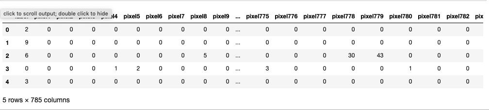
fashion_test_df = pd.read_csv('input/fashion-mnist_test.csv', sep=',')fashion_train_df.head()
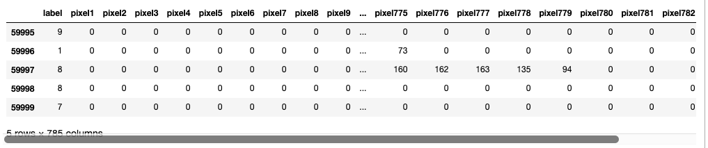
fashion_train_df.tail()
Similarly, for the testing dataset.
fashion_test_df.head()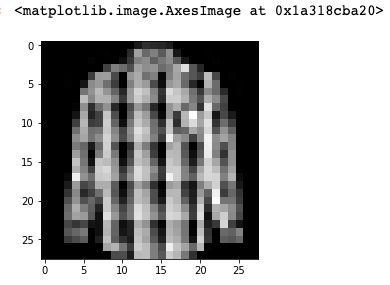
fashion_test_df.tail()i = random.randint(1, 60000)
plt.imshow(training[i, 1:].reshape((28, 28)), cmap='gray')
training = np.array(fashion_train_df, dtype = ‘float32’)
testing = np.array(fashion_test_df, dtype=’float32')i = random.randint(1,60000) # select any random index from 1 to 60,000
plt.imshow( training[i,1:].reshape((28,28)) ) # reshape and plot the imageplt.imshow( training[i,1:].reshape((28,28)) , cmap = 'gray') # reshape and plot the image# Remember the 10 classes decoding is as follows: 0 => T-shirt/top
1 => Trouser
2 => Pullover
3 => Dress
4 => Coat
5 => Sandal
6 => Shirt
7 => Sneaker
8 => Bag
9 => Ankle boot

shirt
W_grid = 15
L_grid = 15# fig, axes = plt.subplots(L_grid, W_grid)
# subplot return the figure object and axes object
# we can use the axes object to plot specific figures at various locationsfig, axes = plt.subplots(L_grid, W_grid, figsize = (17,17))axes = axes.ravel() # flaten the 15 x 15 matrix into 225 arrayn_training = len(training) # get the length of the training dataset# Select a random number from 0 to n_training
for i in np.arange(0, W_grid * L_grid): # create evenly spaces variables# Select a random number
    index = np.random.randint(0, n_training)
    # read and display an image with the selected index
    axes[i].imshow( training[index,1:].reshape((28,28)) )
    axes[i].set_title(training[index,0], fontsize = 8)
    axes[i].axis('off')plt.subplots_adjust(hspace=0.4)
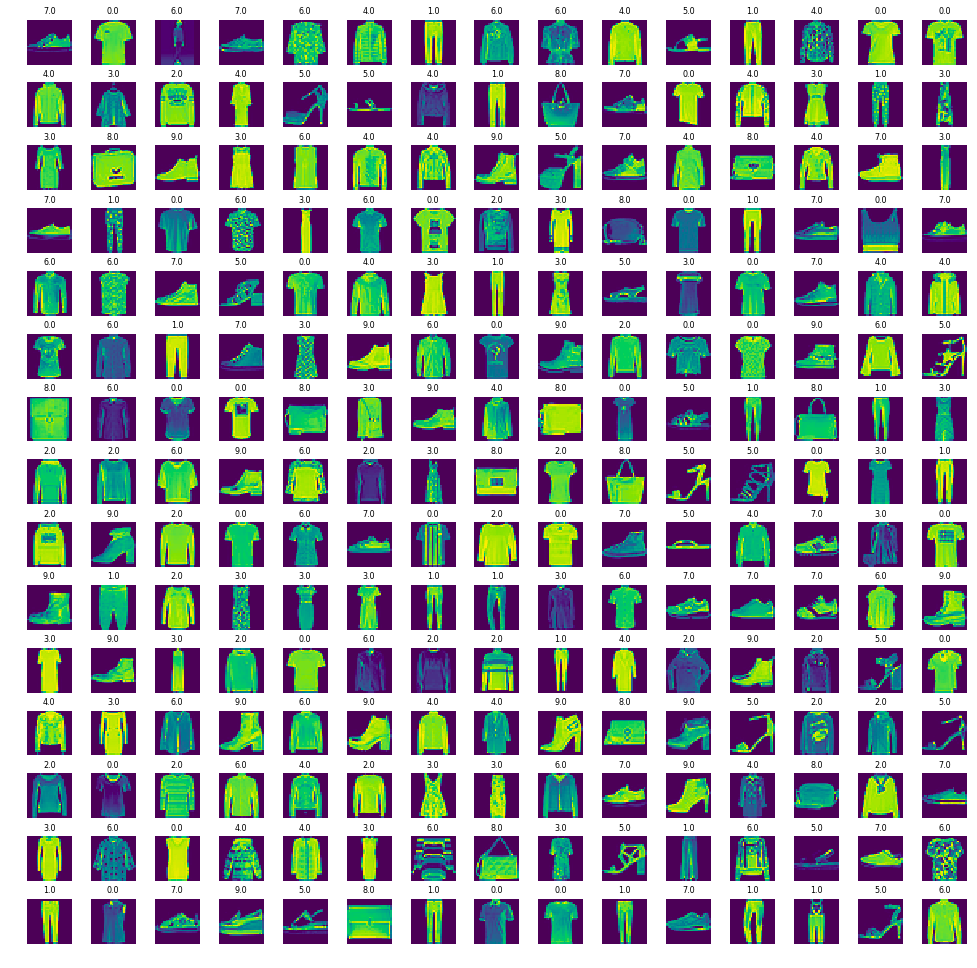
images in a grid format
X_train = training[:, 1:] / 255
y_train = training[:, 0]

X_test = testing[:, 1:] / 255
y_test = testing[:, 0]

# Split the training data into training and validation sets
from sklearn.model_selection import train_test_split

X_train, X_validate, y_train, y_validate = train_test_split(X_train, y_train, test_size=0.2, random_state=12345)X_train = X_train.reshape(X_train.shape[0], 28, 28, 1)
X_test = X_test.reshape(X_test.shape[0], 28, 28, 1)
X_validate = X_validate.reshape(X_validate.shape[0], 28, 28, 1)

import keras
from keras.models import Sequential
from keras.optimizers import Adam
from keras.layers import Conv2D, MaxPooling2D
from keras.layers import Dropout, Flatten, Dense

cnn_model = Sequential()

cnn_model.add(Conv2D(64, 3, 3, input_shape=(28, 28, 1), activation='relu'))
cnn_model.add(MaxPooling2D(pool_size=(2, 2)))
cnn_model.add(Dropout(0.25))

cnn_model.add(Flatten())
cnn_model.add(Dense(output_dim=32, activation='relu'))
cnn_model.add(Dense(output_dim=10, activation='sigmoid'))

cnn_model.compile(loss='sparse_categorical_crossentropy', optimizer=Adam(lr=0.001), metrics=['accuracy'])

epochs = 50
history = cnn_model.fit(X_train, y_train, batch_size=512, nb_epoch=epochs, verbose=1, validation_data=(X_validate, y_validate))
https://www.reddit.com/r/ProgrammerHumor/comments/a8ru4p/machine_learning_be_like/
Model evaluation metrics are used to assess goodness of fit between model and data, to compare different models, in the context of model selection, and to predict how predictions (associated with a specific model and data set) are expected to be accurate
evaluation = cnn_model.evaluate(X_test, y_test)
print('Test Accuracy: {:.3f}'.format(evaluation[1]))predicted_classes = cnn_model.predict_classes(X_test)
# Visualize the predictions
L = 5
W = 5
fig, axes = plt.subplots(L, W, figsize=(12, 12))
axes = axes.ravel()
for i in np.arange(0, L * W):
axes[i].imshow(X_test[i].reshape(28, 28))
axes[i].set_title("Prediction Class = {:0.1f}\nTrue Class = {:0.1f}".format(predicted_classes[i], y_test[i]))
axes[i].axis('off')from sklearn.metrics import confusion_matrix
cm = confusion_matrix(y_test, predicted_classes)
plt.figure(figsize=(14, 10))
sns.heatmap(cm, annot=True)from sklearn.metrics import classification_report
num_classes = 10
target_names = ["Class {}".format(i) for i in range(num_classes)]
print(classification_report(y_test, predicted_classes, target_names=target_names))CNNs are a class of deep learning models specifically designed for image processing. They consist of convolutional layers, pooling layers, and fully connected layers.
- Convolutional Layers: These layers apply filters to extract features from input images. The filters slide over the input image, capturing spatial patterns.
- Pooling Layers: Pooling layers reduce the spatial dimensions of the feature maps, which helps reduce computational complexity.
- Dropout: Dropout layers are used to prevent overfitting.
They randomly deactivate a portion of neurons during training.
- Normalization: Normalizing pixel values to a range between 0 and 1 helps in training convergence.
- Reshaping: Images are reshaped to fit the input size of the neural network.
- Loss Function: The choice of loss function depends on the task. In this project, we use sparse categorical cross-entropy, which is suitable for multi-class classification.
- Optimizer: The Adam optimizer is used with a learning rate of 0.001 for parameter updates.
- Evaluation metrics include accuracy, precision, recall, and F1-score.
- The confusion matrix visually represents the classification results.
- A classification report provides a comprehensive view of model performance.
- Overfitting occurs when the model performs well on the training data but poorly on unseen data. Techniques like dropout layers help prevent overfitting.
- Data augmentation techniques increase the diversity of the training dataset by applying transformations like rotation, scaling, and flipping.
- Finding optimal hyperparameters, such as batch size and number of epochs, is crucial for model performance.
- Transfer learning involves using pre-trained models and fine-tuning them for specific tasks. It can save training time and resources.
- Deep Learning with Keras: Official documentation for the Keras deep learning framework.
- TensorFlow: An open-source machine learning framework that can be used alongside Keras for more advanced deep learning projects.
- Scikit-learn: A powerful machine learning library for various tasks, including data preprocessing and model evaluation.
- Matplotlib: A popular Python library for creating visualizations and plots.
- Seaborn: An easy-to-use Python data visualization library that works well with Matplotlib.
- Reddit - Machine Learning Humor: A lighthearted take on the complexities of machine learning.
- Sajjad Salaria - Project Lead
This project is licensed under the MIT License - see the LICENSE file for details.
Special thanks to the authors and contributors of the following resources: