2_3_step11_16
All steps can be sequentially processed using a batch script.
For more details of the commands, use -h option to see the usage.
LiCSBAS11_check_unw.py -d ifgdir [-t tsadir] [-c coh_thre] [-u unw_thre]

 -d  Path to the GEOCml* dir containing stack of unw data.
 -t  Path to the output TS_GEOCml* dir. (Default: TS_GEOCml*)
 -c  Threshold of average coherence (Default: 0.05)
 -u  Threshold of coverage of unw data (Default: 0.3)
This script checks quality of unw data and identifies bad interferograms based on average coherence and coverage of the unw data. This also prepares a time series working directory (overwrite if already exists).
LiCSBAS12_loop_closure.py -d ifgdir [-t tsadir] [-l loop_thre] [--multi_prime]
 [--rm_ifg_list file] [--n_para int]

 -d  Path to the GEOCml* dir containing stack of unw data.
 -t  Path to the output TS_GEOCml* dir. (Default: TS_GEOCml*)
 -l  Threshold of RMS of loop phase (Default: 1.5 rad)
 --multi_prime  Multi Prime mode (take into account bias in loop)
 --rm_ifg_list  Manually remove ifgs listed in a file
 --n_para  Number of parallel processing (Default: # of usable CPU)
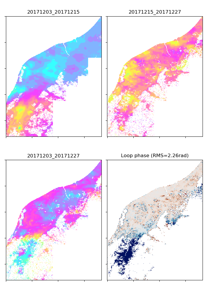
This script identifies bad unw by checking loop closure. A preliminary reference point that has all valid unw data and the smallest RMS of loop phases is also determined.
LiCSBAS13_sb_inv.py -d ifgdir [-t tsadir] [--inv_alg LS|WLS] [--mem_size float] [--gamma float]
  [--n_para int] [--n_unw_r_thre float] [--keep_incfile] [--gpu]

 -d  Path to the GEOCml* dir containing stack of unw data
 -t  Path to the output TS_GEOCml* dir.
 --inv_alg    Inversion algolism (Default: LS)
   LS :       NSBAS Least Square with no weight
   WLS:       NSBAS Weighted Least Square (not well tested)
              Weight (variance) is calculated by (1-coh**2)/(2*coh**2)
 --mem_size   Max memory size for each patch in MB. (Default: 8000)
 --gamma      Gamma value for NSBAS inversion (Default: 0.0001)
 --n_para     Number of parallel processing (Default: # of usable CPU)
 --n_unw_r_thre
     Threshold of n_unw (number of used unwrap data)
     (Note this value is ratio to the number of images; i.e., 1.5*n_im)
     Larger number (e.g. 2.5) makes processing faster but result sparser.
     (Default: 1 and 0.5 for C- and L-band, respectively)
 --keep_incfile
     Not remove inc and resid files (Default: remove them)
 --gpu        Use GPU (Need cupy module)
This script inverts the SB network of unw to obtain the time series and velocity using NSBAS (López-Quiroz et al., 2009; Doin et al., 2011) approach. A stable reference point is determined after the inversion. RMS of the time series wrt median among all points is calculated for each point. Then the point with minimum RMS and minimum n_gap is selected as new stable reference point.
LiCSBAS14_vel_std.py -t tsadir [--mem_size float] [--gpu]

 -t  Path to the TS_GEOCml* dir.
 --mem_size   Max memory size for each patch in MB. (Default: 4000)
 --gpu        Use GPU (Need cupy module)
This script calculates the standard deviation of the velocity by the bootstrap method and STC (spatio-temporal consistency; Hanssen et al., 2008).
LiCSBAS15_mask_ts.py -t tsadir [-c coh_thre] [-u n_unw_r_thre] [-v vstd_thre]
  [-T maxTlen_thre] [-g n_gap_thre] [-s stc_thre] [-i n_ifg_noloop_thre]
  [-l n_loop_err_thre] [-r resid_rms_thre] [--vmin float] [--vmax float]
  [--keep_isolated] [--noautoadjust]

 -t  Path to the TS_GEOCml* dir.
 -c  Threshold of coh_avg (average coherence)
 -u  Threshold of n_unw (number of used unwrap data)
     (Note this value is ratio to the number of images; i.e., 1.5*n_im)
 -v  Threshold of vstd (std of the velocity (mm/yr))
 -T  Threshold of maxTlen (max time length of connected network (year))
 -g  Threshold of n_gap (number of gaps in network)
 -s  Threshold of stc (spatio-temporal consistency (mm))
 -i  Threshold of n_ifg_noloop (number of ifgs with no loop)
 -l  Threshold of n_loop_err (number of loop_err)
 -r  Threshold of resid_rms (RMS of residuals in inversion (mm))
 --v[min|max]  Min|Max value for output figure of velocity (Default: auto)
 --keep_isolated  Keep (not mask) isolated pixels
                  (Default: they are masked by stc)
 --noautoadjust  Do not auto adjust threshold when all pixels are masked
                 (Default: do auto adjust)

 Default thresholds for L-band:
   C-band : -c 0.05 -u 1.5 -v 100 -T 1 -g 10 -s 5  -i 50 -l 5 -r 2
   L-band : -c 0.01 -u 1   -v 200 -T 1 -g 1  -s 10 -i 50 -l 1 -r 10
This script makes a mask for time series using several noise indices. The pixel is masked if any of the values of the noise indices for a pixel is worse (larger or smaller) than a specified threshold.
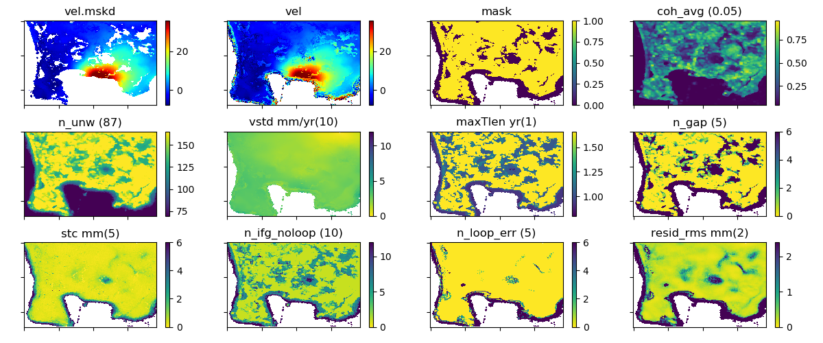
| Noise index | Meaning |
|---|---|
| coh_avg | Average value of the interferometric coherence across the stack (0–1). |
| n_unw | Number of unwrapped data used in the time series calculation. (Note: the argument is ratio to the number of images; i.e., if 1.5, n_unw=1.5*n_im) |
| vstd | Standard deviation of the velocity (mm/yr) estimated in Step 1-4. |
| maxTlen | Maximum time length of the connected network (years). The larger the value, the better the precision in the velocity estimate. |
| n_gap | Number of gaps in the interferogram network and time series breaks. |
| stc | Spatio-temporal consistency (mm) (Hanssen et al., 2008, Terrafirma), estimated in Step 1-4. |
| n_ifg_noloop | Number of interferograms with no loops that cannot be checked by the loop closure and possibly have unidentified unwrapping errors. |
| n_loop_err | Number of the unclosed loops after the network refinement in Step 1-2. |
| resid_rms | RMS of residuals in the small baseline (SB) inversion (mm). |
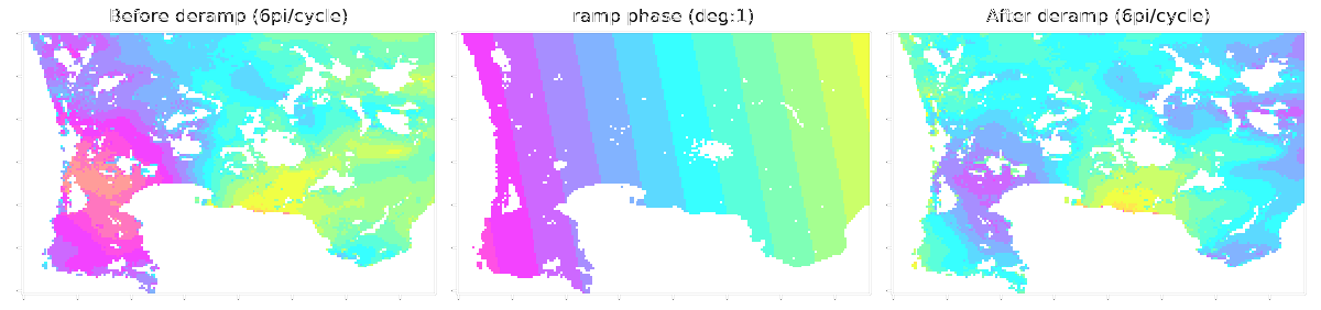
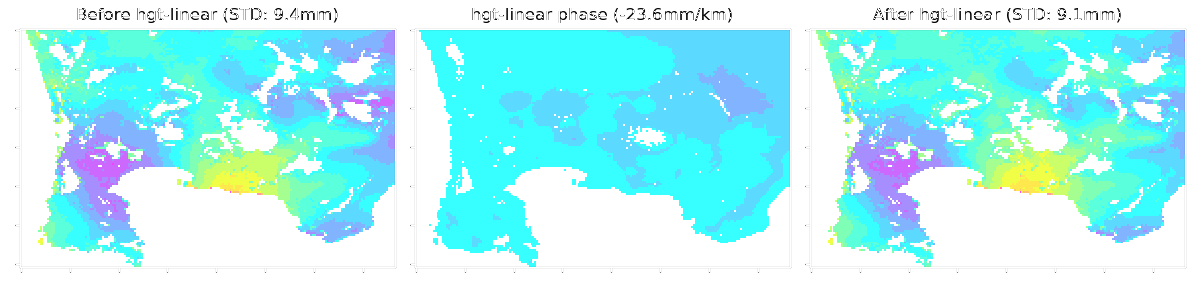
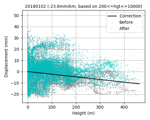
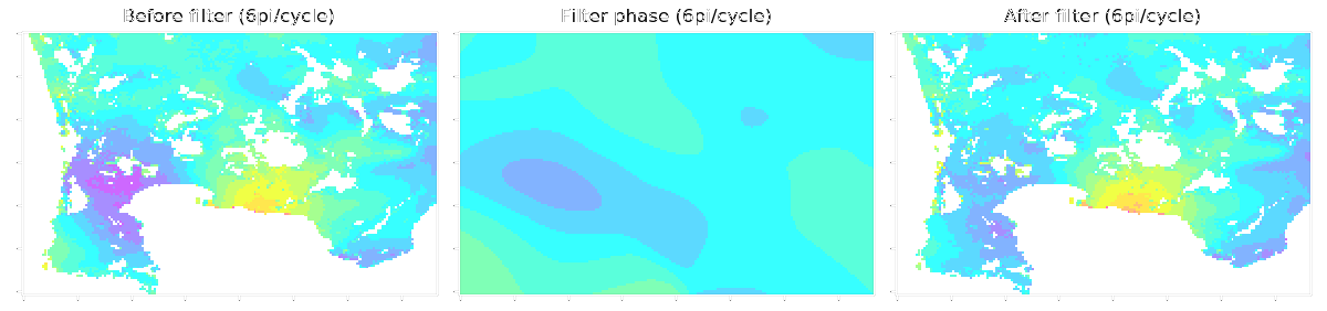
LiCSBAS16_filt_ts.py -t tsadir [-s filtwidth_km] [-y filtwidth_yr] [-r deg]
 [--hgt_linear] [--hgt_min int] [--hgt_max int] [--nomask] [--n_para int]
 [--range x1:x2/y1:y2 | --range_geo lon1/lon2/lat1/lat2]
 [--ex_range x1:x2/y1:y2 | --ex_range_geo lon1/lon2/lat1/lat2]

 -t  Path to the TS_GEOCml* dir.
 -s  Width of spatial filter in km (Default: 2 km)
 -y  Width of temporal filter in yr (Default: auto, avg_interval*3)
 -r  Degree of deramp [1, bl, 2] (Default: no deramp)
     1: 1d ramp, bl: bilinear, 2: 2d polynomial
 --hgt_linear Subtract topography-correlated component using a linear method
              (Default: Not apply)
 --hgt_min    Minumum hgt to take into account in hgt-linear (Default: 200m)
 --hgt_max    Maximum hgt to take into account in hgt-linear (Default: 10000m, no effect)
 --nomask     Apply filter to unmasked data (Default: apply to masked)
 --n_para     Number of parallel processing (Default: # of usable CPU)
 --range      Range used in deramp and hgt_linear. Index starts from 0.
              0 for x2/y2 means all. (i.e., 0:0/0:0 means whole area).
 --range_geo  Range used in deramp and hgt_linear in geographical coordinates (deg).
 --ex_range   Range EXCLUDED in deramp and hgt_linear. Index starts from 0.
              0 for x2/y2 means all. (i.e., 0:0/0:0 means whole area).
 --ex_range_geo  Range EXCLUDED in deramp and hgt_linear in geographical
                 coordinates (deg).

Note: Spatial filter consume large memory. If the processing is stacked, try
 - --n_para 1
 - Indicate small filtwidth_km for -s option
 - Reduce data size in step02 or step05
This script applies spatio-temporal filter (HP in time and LP in space with gaussian kernel, same as StaMPS) to the time series of displacement. Deramping (1D, bilinear, or 2D polynomial) can also be applied if -r option is used. Topography-correlated components (linear with elevation) can also be subtracted with --hgt_linear option simultaneously with deramping before spatio-temporal filtering. The impact of filtering (deramp and linear elevation as well) can be visually checked by showing 16filt*/*png. A stable reference point is determined after the filtering as well as Step 1-3.