-
Notifications
You must be signed in to change notification settings - Fork 3
Modflow example
The hypothetical example is described in great detail in the supplemental material of our paper (the link will be added)
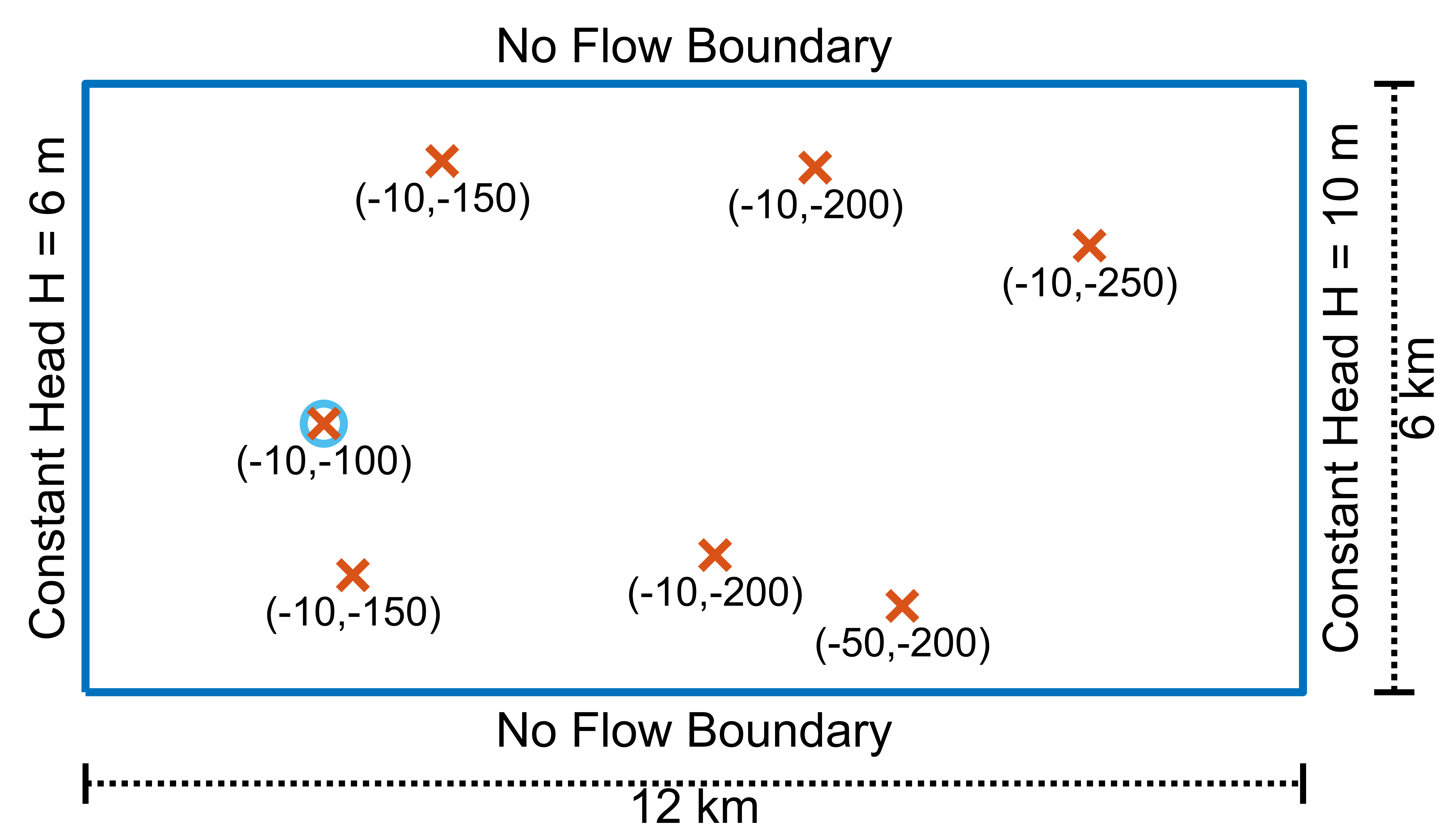
The domain of this example is a rectangular box with dimensions 12 x 6 km.

The polygon must be counter clockwise oriented.
domain_poly = [0 0;12000 0;12000 6000; 0 6000];
fid = fopen('mp_test_outline.ich', 'w');
fprintf(fid, '%d %d\n', [size(domain_poly,1) 1]);
fprintf(fid, '%.1f %.1f\n', domain_poly');
fclose(fid);
The top varies linearly from 6 m at x = 0 to 10 m at x = 12 km. To define the top we will use the MESH2D option where we set the elevation at the mesh nodes and provide information on the mesh connectivity. Here we will use a mesh with 1 element. We will offset the nodes by 1 m to avoid situations where an interpolated point lies on the edge but due to numerical imprecision is found outside. Note that the radius parameter was set to 12000 so that all points of the domain are within the search radius from the barycenter of the single element.
a = (10-6)/12000; % slope
b = 6; % intercept
ftop = @(x) a.*x+b;
d = [-1 -1;12001 -1;12001 6001; -1 6001];
fid = fopen('mp_test_top.ich', 'w');
fprintf(fid, 'MESH2D\n');
fprintf(fid, '%d %d %.2f\n', [4 1 12000]);
fprintf(fid, '%.1f %.1f %.7f\n', [d ftop(d(:,1))]');
fprintf(fid, '%d %d %d %d\n', [1 2 3 4]);
fclose(fid);
The bottom elevation is constant therefore we can simply pass the numeric value instead of a file
BottomFile = -300
In this example we will use the FACE interpolation option of Ichnos which requires to define a 2D mesh.
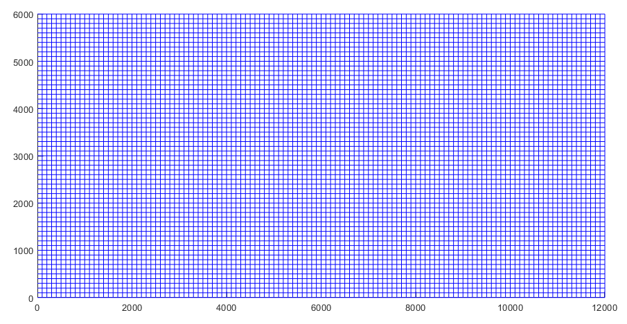
In a real application the mesh maybe provided as a shapefile e.g. CVHM2. Here because the mesh is very simple we will create it via code. The mesh requires three files: i) node file, ii) mesh file and iii) elevation file.
[NDX, NDY] = meshgrid(0:100:12000,0:100:6000);
NDY = flipud(NDY);
[IX, IY] = meshgrid(1:121,1:61);
linind = sub2ind(size(IX),IY,IX);
idx = reshape(linind,121*61,1);
ND = [NDX(idx) NDY(idx)];
Print the file
fid = fopen('mp_test_Node.ich','w');
fprintf(fid,'%.2f %.2f\n', ND');
fclose(fid);
msh = nan(7200,4);
cnt = 1;
for ii = 1:size(linind,1)-1
    for jj = 1:size(linind,2)-1
        msh(cnt,:) = [linind(ii,jj) linind(ii+1,jj) linind(ii+1,jj+1) linind(ii,jj+1)];
        cnt = cnt + 1;
    end
end
Print the mesh file. Note that the mesh file expects the indices to start at 1 not 0. The fifth column is the processor id. The mesh indices must be oriented in counter clockwise order. The above loop setups the elements so that they are all counter clockwise.
fid = fopen('mp_test_Mesh.ich','w');
fprintf(fid,'%d %d %d %d %d\n', [msh zeros(size(msh,1),1)]');
fclose(fid);

Assign elevation to the nodes
top_elev = ftop(ND(:,1));
bot_elev = -300*ones(size(ND,1),1);
Elev = nan(size(ND,1), 21);
t = linspace(0,1,21);
for ii = 1:length(t)
    Elev(:,ii) = top_elev.*(1-t(ii)) + bot_elev.*t(ii);
end
Print the elevation file
fid = fopen(fullfile(input_dir,'mp_test_Elev.ich'),'w');
fprintf(fid,['%.2f' repmat(' %.2f',1,size(Elev,2) - 1) '\n'], Elev');
fclose(fid);
The Modflow simulation generates a cell by cell file which contains the flow information that we will use it to derive the groundwater velocity. The *.cbc file of our example can be downloaded from this link. To read it using matlab we use the readCVHMcbc.m which is provided as gist.
Read the cell by cell file
cbc = readCVHMcbc('mp_test02.cbc');
The output of this file at the time of writing is the following. Despite the warning the script has read correctly the flow information
Reading CONSTANT HEAD for Period 1
Reading FLOW RIGHT FACE for Period 1
Reading FLOW FRONT FACE for Period 1
Reading FLOW LOWER FACE for Period 1
Reading WELLS for Period 1
Warning: ITYPE == 5 and NVAL > 1 not implemented yet
> In readCVHMcbc (line 43)
Reading RECHARGE for Period 1
Reading  for Period
According to Modflow Flow definition :
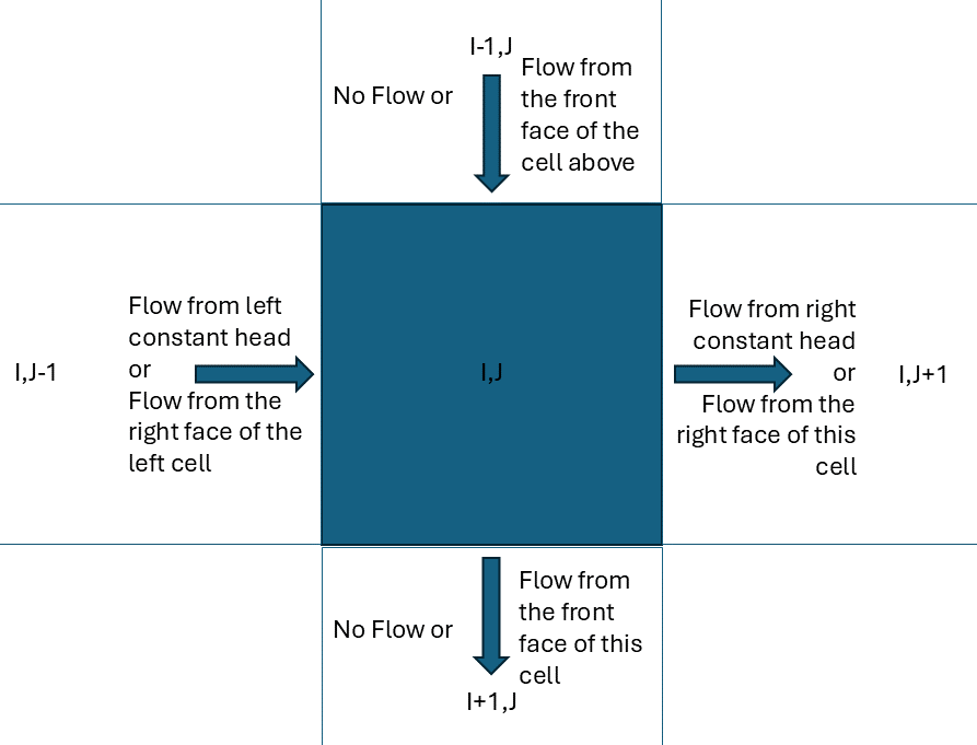
- FLOW RIGHT FACE: flow between the cells [J, I, K] and [J+1, I, K]
- FLOW FRONT FACE: flow between the cells [J, I, K] and [J, I+1, K]
- FLOW LOWER FACE: flow between the cells [J, I, K] and [J, I, K+1]
To assign the horizontal face velocities in our hypothetical example we will use the following guide

The CONSTANT HEAD flow contains the flow from the west and east boundary conditions, the FLOW FACES give the flow between the cells while the north and south boundary flows are all set to zero. The LOWER flow contains the flow between the layers while for the top we will use the groundwater recharge.
The next loop identifies the unique faces in the grid and makes a list of the flows. First initialize a few variables
bcx = (ND(msh(:,1),1) + ND(msh(:,2),1) + ND(msh(:,3),1) + ND(msh(:,4),1))/4;
bcy = (ND(msh(:,1),2) + ND(msh(:,2),2) + ND(msh(:,3),2) + ND(msh(:,4),2))/4;
clear FACEFLOWS
face_node_ids = zeros(15000,2);
face_vel_values = zeros(15000,20);
face_vert_vel_values = zeros(7200,21);
face_vel_ids = zeros(size(msh,1),4);
cnt_fc = 0;
bcx bcy holds the barycenters of the mesh elements. face_node_ids holds the node ids of the unique faces. face_vel_values will be populated with the horizontal flow values and face_vert_vel_values with the vertical flow values. The columns correspond to layers. Last the face_vel_ids will containts the face ids as descibed in the documentation. These contain the row where the face values are in the face_vel_values variable.
The next following loop is quite lengthy and we break it into sections to discuss the logic. We provide the same code here without the comments
First we will loop through the rows and columns and store into FACEFLOWS all the flows associated with the row,col cell. Note that when col is 1 or 120 we store the constant head flows too.
for row = 1:60
    for col = 1:120
        tmp_face_values = zeros(4,20);
        if col == 1 || col == 120
            idx = find(cbc{1,1}{1,2}(:,2) == row & cbc{1,1}{1,2}(:,3) == col);
            FACEFLOWS(row,col).CNSTHD = cbc{1,1}{1,2}(idx,4);
        end
        FACEFLOWS(row,col).FRONT = reshape(cbc{1,1}{3,2}(row,col,:),20,1);
        FACEFLOWS(row,col).RIGHT = reshape(cbc{1,1}{2,2}(row,col,:),20,1);
        FACEFLOWS(row,col).VERT = [cbc{1,1}{6,2}(row,col); reshape(cbc{1,1}{4,2}(row,col,:),20,1)];
Next we populate the temporary variable tmp_face_values with the face flows of the row,col cell. The variable has 4 rows one for each element side. When we built the mesh (see above) the 1st, 2nd, 3rd and 4th face correspond to the west, south, east, north face of the cell. Accordingly each row of the tmp_face_values corresponds to the 1st, 2nd, 3rd and 4th face.
        if col == 1
            tmp_face_values(1,:) = FACEFLOWS(row,col).CNSTHD';
        else
            tmp_face_values(1,:) = FACEFLOWS(row,col-1).RIGHT';
        end
        if row == 60
            tmp_face_values(2,:) = zeros(1,20);
        else
            tmp_face_values(2,:) = FACEFLOWS(row,col).FRONT';
        end
        if col == 120
            tmp_face_values(3,:) = FACEFLOWS(row,col).CNSTHD';
        else
            tmp_face_values(3,:) = FACEFLOWS(row,col).RIGHT';
        end
        if row == 1
            tmp_face_values(4,:) = zeros(1,20);
        else
            tmp_face_values(4,:) = FACEFLOWS(row-1,col).FRONT';
        end
The following part of the loop identifies the row index dd of the msh that corresponds to the row, col cell. We do this by calculating the distance between the barycenter xx,yy of the row,col cell and all barycenters bcx,bcy of the msh. The minimum distance should be almost zero which indicates the element that corresponds to the row,col cell. This should always find an element. Once we know the mesh index we populate the vertical flows.
        xx = (NDX(row,col) + NDX(row,col+1))/2;
        yy = (NDY(row,col) + NDY(row+1,col))/2;
        [cc, dd] = min(sqrt((xx - bcx).^2 + (yy - bcy).^2));
        if cc < 0.01
            FACEFLOWS(row,col).meshID = dd;
            FACEFLOWS(row,col).meshNDid = msh(dd,:);
        else
            error('The code should never reach here')
        end

        face_vert_vel_values(dd,:) = FACEFLOWS(row,col).VERT';
If this is the first cell row=1, col=1 then we simply assigned the face flows to the variables.
        if cnt_fc == 0
            face_node_ids(1:4,:) = [msh(dd,1:2); msh(dd,2:3);msh(dd,3:4); msh(dd,[4 1])];
            face_vel_ids(dd,:) = [-1 2 3 -4];
            face_vel_values(1:4,:) = tmp_face_values;
            cnt_fc = 4;
        else
If the face_node_ids is not empty we need to loop though each face and test if the face is already included in the list. The following code assigns the node ids to ida, idb and checks if the face_node_ids containts a face with those ids. Since we do not know if the face in face_node_ids is written as [ida idb] or [idb ida] we test the first and if its empty we test the second option.
            for ii = 1:4
                ida = msh(dd,ii);
                if ii == 4
                    idb = msh(dd,1);
                else
                    idb = msh(dd,ii+1);
                end
                fc_idx = find(ida == face_node_ids(1:cnt_fc,1) & idb == face_node_ids(1:cnt_fc,2));
                if isempty(fc_idx)
                    fc_idx = find(idb == face_node_ids(1:cnt_fc,1) & ida == face_node_ids(1:cnt_fc,2));
                end
If the face is not in the list add a new face in the variables.
                if isempty(fc_idx)
                    cnt_fc = cnt_fc + 1;
                    face_node_ids(cnt_fc,:) = [ida idb];
                    face_vel_values(cnt_fc,:) = tmp_face_values(ii,:);
                    face_vel_ids(dd,ii) = cnt_fc;
If the face is already in the list we add the id (e.g. the row in the face_node_ids variable) to the element
                else
                    face_vel_ids(dd,ii) = fc_idx;
                end
Last we reverse the signs of the 1st and 4th face (see more)
                if ii == 1 || ii == 4
                    face_vel_ids(dd,ii) = -face_vel_ids(dd,ii);
                end
            end
        end
    end
end
face_node_ids(cnt_fc+1:end,:) = [];
face_vel_values(cnt_fc+1:end,:) = [];
We can now print the face id file
fid = fopen('mp_test_faceIds.ich','w');
fprintf(fid,'%d %d %d %d\n', face_vel_ids');
fclose(fid);
The velocities that we have assembled that far are in face_node_ids which gives us the node ids. First we compute the thickness of the face at each face node and layer and then calculate the area with the trapezoid rule using as height the cell size which is 100 m.
ida_thickness = abs(diff(Elev(face_node_ids(:,1),:),1,2));
idb_thickness = abs(diff(Elev(face_node_ids(:,2),:),1,2));
face_area = (ida_thickness + idb_thickness)*100/2;
face_vel_values_m = face_vel_values./face_area;
face_vert_vel_values_m = face_vert_vel_values/(100*100);
Before we print the velocities into files lets examine the velocity for one cell. Note that this is for illustration only and it is not needed for the file preparation.
We are going to example the velocities of the cell with (row,col,lay)=(35,23,6) and
r = 35;c = 23;l = 6;
FACEFLOWS(r,c).meshID
face_vel_ids(FACEFLOWS(r,c).meshID,:)
face_vel_values_m(abs(face_vel_ids(FACEFLOWS(r,c).meshID,:)),6)*1000
The outcome of this is
4103
-8359	8360	8361	-8119
14.1919
-17.0996
18.0779
-21.2955
where 4103 is the element id for the cell (35,23), the next line are the rows of the face velocities that correspond to the particular faces and the remaining lines are the velocity values multilied by 1000.
- 1st face (west): The velocity of the first face has magnitude equal to 14.1919 and the direction is towards the element since index -8359 is negative
- 2nd face (south): The velocity of the second face is listed as outflow. However the magnitude is -17.0996, which is negative therefore this velocity is also inflow.
- 3rd face (east): The velocity of this face is outflow because both the face is is positive, which indicates outflow and the magnitude is positive (18.0779) which means that the direction is the same as the face indicates
- 4th face (north): The fourth face has negative index which means inflow however this is reversed by the negative sign of the velocity magnitute
The positive vertical velocities in Modflow denote downward movement. However Ichnos assumes positive the upward movement therefore we have to reverse the signs
face_vert_vel_values_m = -1*face_vert_vel_values_m;
Last we print the velocities. For the FACE interpolation option the horizontal and vertical velocities are printed either in different files or different datasets. In either case we have to reformat them
VHOR = reshape(face_vel_values_m,size(face_vel_values_m,1)*size(face_vel_values_m,2),1);
VVER = reshape(face_vert_vel_values_m,size(face_vert_vel_values_m,1)*size(face_vert_vel_values_m,2),1);
The VHOR and VVER variables have nFaces*nLayers and nElements*(nLayers+1) rows respectively and 1 column. If the velocities were transient then for each time step we would add a column.
For ascii files we print two files as follows
fid = fopen('mp_test_vel_VHOR_000.ich','w');
fprintf(fid,'%.7e\n', VHOR');
fclose(fid);

fid = fopen('mp_test_vel_VVER_000.ich','w');
fprintf(fid,'%.7e\n', VVER');
fclose(fid);
For HDF5 the velocities are printed under different datasets
fname = fullfile('mp_test_vel_000.h5');
h5create(fname,'/VHOR',[size(VHOR,1) size(VHOR,2)], 'Datatype','single');
h5write(fname, '/VHOR', VHOR);
h5create(fname,'/VVER',[size(VVER,1) size(VVER,2)], 'Datatype','single');
h5write(fname, '/VVER', VVER);
In this simulation we will release 180 particles from the 7 wells of the model distributed into 30 layers within 9.5 m radius from the well position (see more).
wells = [3516.248 5237.65816 -10 -150;...
         7192.507 5173.802 -10 -200; ...
         9896.432 4403.791 -10 -250; ...
         8051.6 850.974 -50 -200; ...
         6204.278 1352.196 -10 -200; ...
         2635.606 1156.060 -10 -150; ...
         2348.787 2648.002 -10 -100];
fid = fopen('mp_test_wells.ich','w');
fprintf(fid,'%d %d %.2f\n',[180 30 9.5]);
fprintf(fid, '%d %.5f  %.5f  %.2f  %.2f 0\n', [(1:7)' wells]');
fclose(fid);
Here we describe the options for the main and velocity configuration file
[Velocity]
XYZType = MESH2D
Type = DETRM
ConfigFile = mp_test_vf.ini
[Domain]
Outline = mp_test_outline.ich
TopFile = mp_test_top.ich
BottomFile = -300
ProcessorPolys =
[StepConfig]
Method = PECE
Direction = -1
StepSize = 50
StepSizeTime = 100000
nSteps = 5
nStepsTime = 0
minExitStepSize = 1
[PECE]
Order = 4
Tolerance = 0.2
[StoppingCriteria]
MaxIterationsPerStreamline = 3000
MaxProcessorExchanges = 50
AgeLimit = -1
StuckIter = 10
AttractFile =
AttractRadius = 30
[InputOutput]
ParticleFile =
WellFile = mp_test_wells.ich
OutputFile = path/to/mp_test_out
PrintH5 = 1
PrintASCII = 1
ParticlesInParallel = 5000
GatherOneFile = 0
[Other]
Version = 0.4.10
Nrealizations = 1
nThreads = 1
RunAsThread = 1
OutFreq = 20
[Velocity]
Prefix = mp_test_vel_
LeadingZeros = 3
Suffix = .ich
Type = DETRM
TimeStepFile =
TimeInterp =
RepeatTime = 0
Multiplier = 1
The option Suffix = .ich will make ichnos to read the ascii files. Alternatively we can pass Suffix = .h5 which will make the code to read the hdf5 files. In general reading HDF5 is much faster.
[MESH2D]
NodeFile = mp_test_Node.ich
MeshFile = mp_test_Mesh.ich
ElevationFile = mp_test_Elev.ich
FaceIdFile = mp_test_faceIds.ich
Nlayers = 20
INTERP = FACE
[Porosity]
Value = 0.1
Ichnos is a concole application. To run it execute the following in a terminal. (e.g windows powershell)
ichnos.exe -c .\mp_test_config.ini
This will execute the tracing using a sinlge process and the output log of the simulation will be similar to the following
Ichnos started at Wed Aug 28 10:00:47 2024

Ichnos will run using 1 processors
Reading input data...
--> Configuration file: .\mp_test_config.ini
        Reading XYZ data from mp_test_vf.ini...
        Point Set Building time: 0.0015035
--> Velocity configuration file: mp_test_vf.ini
        Read Velocity in : 0.0516712
Tracing particles...
-20 % |253 of 1260
-40 % |505 of 1260
-60 % |757 of 1260
-80 % |1009 of 1260
Total simulation Time : 1.66174
Ichnos Finished at Wed Aug 28 10:00:53 2024
The output of this run is a single file which has the prefix OutputFile = path/to/mp_test_out
We can read this file in matlab using the readICHNOStraj function which is part of our gwtools repository.
Depending the flags PrintH5 = 1 and PrintASCII = 1 we can print the output to hdf5, ascii or both.
To read the ascii we can do in one line but we use tic/toc to count the reading time. The following required about 77 seconds
tic
S = readICHNOStraj('mp_test_out_iter_0000.traj');
toc
For HDF5 we can use the same command but this time it took 3.4 seconds to read.
tic
S = readICHNOStraj('mp_test_out_iter_0000.h5');
toc
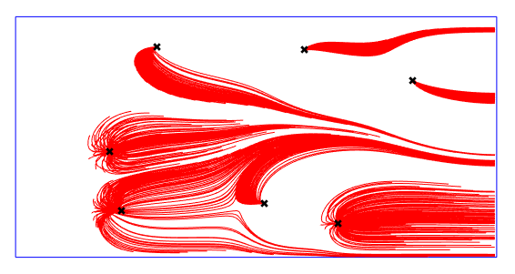
Finally lets visualize the streamlines. The output structure S is discussed here.
figure()
clf
plot(domain_poly([1:4 1],1),domain_poly([1:4 1],2),'b')
hold on
for ii = 1:length(S)
    plot(S(ii,1).p(:,1),S(ii,1).p(:,2),'r')
end
axis equal
plot(wells(:,1),wells(:,2),'xk','MarkerSize',7,'LineWidth',2)
axis off

Notice that the simulation was executed in 1.66 seconds. In such a small test case there is no essential benefit to run it as a multi process. However if there is a need to run e.g millions of particles we can speed up the simulation by distributing the particles into different processors. This does not involve any further step during the setup files
To run as multicore process we change the console command as follows:
C:\"Program Files\Microsoft MPI"\Bin\mpiexec.exe -n 4 ichnos.exe -c .\mp_test_config.ini
where -n 4 is the number of cores to use.
As we can see from the console output each core reads the configuration file and all the input files and they all build the required sets for the simulation.
Then the 1260 particles are split into 4 groups of 315 which are traced concurrently. Each core tracks its own progress and reports it. Overall the simulation time is now around 0.5 seconds
--> Configuration file: .\mp_test_config.ini
--> Configuration file: .\mp_test_config.ini
--> Configuration file: .\mp_test_config.ini
Ichnos started at Wed Aug 28 10:31:26 2024

Ichnos will run using 4 processors
Reading input data...
--> Configuration file: .\mp_test_config.ini
        Reading XYZ data from mp_test_vf.ini...
        Point Set Building time: 0.0015831
        Point Set Building time: 0.0013765
        Point Set Building time: 0.0012532
        Point Set Building time: 0.0017601
--> Velocity configuration file: mp_test_vf.ini
        Read Velocity in : 0.0371177
        Read Velocity in : 0.0371967
        Read Velocity in : 0.0383967
        Read Velocity in : 0.0385424
Tracing particles...
-20 % |64 of 315
-20 % |64 of 315
-20 % |64 of 315
-20 % |64 of 315
-40 % |127 of 315
-40 % |127 of 315
-40 % |127 of 315
-40 % |127 of 315
-60 % |190 of 315
-60 % |190 of 315
-60 % |190 of 315
-60 % |190 of 315
-80 % |253 of 315
-80 % |253 of 315
-80 % |253 of 315
-80 % |253 of 315
Total simulation Time : 0.511868
Total simulation Time : 0.530232
Total simulation Time : 0.516778
Total simulation Time : 0.523475
Ichnos Finished at Wed Aug 28 10:31:28 2024
In multicore simulations the streamlines have been printed into multiple files
Notice that there is a _proc_#### appended to each file.
We can read and visualize them in a similar way.
cl_ord = colororder;
figure()
clf
plot(domain_poly([1:4 1],1),domain_poly([1:4 1],2),'b')
hold on
for ii = 1:4
    S(ii,1).Data = readICHNOStraj(['mp_test_out_iter_0000_iproc_' num2str(ii-1,'%04d') '.h5']);

    for j = 1:length(S(ii,1).Data)
        plot(S(ii,1).Data(j,1).p(:,1),S(ii,1).Data(j,1).p(:,2),'Color',cl_ord(ii+1,:))
    end
end
axis equal
plot(wells(:,1),wells(:,2),'xk','MarkerSize',7,'LineWidth',2)
axis off
In the following we plot each processor streamlines with different color.