-
Notifications
You must be signed in to change notification settings - Fork 3
Simple Example
In this example we will demonstrate how to prepare the input files for the various interpolation options that are currently available.
This example is totally fictional and the velocity data are read from a file that we have prepared and contain some sort of random data based on a simple perlin noise generator. Don't worry if that last part it is not clear.
The domain is rectanglular with dimensions 300 x 300 x 10 m.
First we need to define the domain outline in the 2D coordinate space.
domain_poly = [0 0;300 0;300 300; 0 300];
Print the Ichnos input file
fid = fopen('simple_outline.ich', 'w');
fprintf(fid, '%d %d\n', [size(domain_poly,1) 1]);
fprintf(fid, '%.1f %.1f\n', domain_poly');
fclose(fid);
For simplicity we will keep the top and bottom elevations constant. Therefore we can define under the Domain section the following options:
TopFile = 10
BottomFile = 0
For CLOUD based interpolation the following mesh files are not needed.
The MESH2D requires the preparation of 3 files:
i) Node file,
ii) Mesh file,
iii) Elevation file.
First we are going to define the discretization options or density of mesh points/elements
nNodesX = 6;
nNodesY = 5;
nNodesZ = 3;
Nodes
[NDX, NDY] = meshgrid(linspace(0,300,nNodesX),linspace(0,300,nNodesY));
NDY = flipud(NDY);
[IX, IY] = meshgrid(1:nNodesX,1:nNodesY);
linind = sub2ind(size(IX),IY,IX);
idx = reshape(linind,nNodesX*nNodesY,1);
ND = [NDX(idx) NDY(idx)];
Print node file
fid = fopen('Simple_Node.ich','w');
fprintf(fid,'%.2f %.2f\n', ND');
fclose(fid);
msh = nan((nNodesX-1)*(nNodesY-1),4);
cnt = 1;
for ii = 1:size(linind,1)-1
    for jj = 1:size(linind,2)-1
        msh(cnt,:) = [linind(ii,jj) linind(ii+1,jj) linind(ii+1,jj+1) linind(ii,jj+1)];
        cnt = cnt + 1;
    end
end
The elements must be oriented in counter clockwise direction. To check this we do the following which should result all zeros
for ii = 1:9
    c(ii,1) = ispolycw(ND(msh(ii,:),1), ND(msh(ii,:),2));
end
Print the mesh file
fid = fopen('Simple_Mesh.ich','w');
fprintf(fid,'%d %d %d %d %d\n', [msh zeros(size(msh,1),1)]');
fclose(fid);
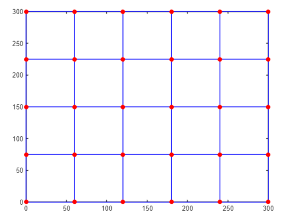
Let's visualize the mesh
figure()
clf
plot(domain_poly([1:4 1],1), domain_poly([1:4 1],2))
hold on
for ii = 1:size(msh)
    plot(ND(msh(ii,[1:4 1]),1),ND(msh(ii,[1:4 1]),2),'b')
end
plot(ND(:,1), ND(:,2),'.r','MarkerSize',20)

Elev = repmat(linspace(10,0,nNodesZ),size(ND,1),1);
Print the file
fid = fopen('Simple_Elev.ich','w');
fprintf(fid,['%.2f' repmat(' %.2f',1,size(Elev,2) - 1) '\n'], Elev');
fclose(fid);
The velocity is based on a random perlin noise. The velocity data can be read from the file test_cloudall_0.dat. In the following we read it as table, rename the columns and transform the coordinates appropriately.
v = readtable('G:\UCDAVIS\ichnos\ichnos_hou\ichnos\test_cloudall_0.dat');
v = renamevars(v,["Var1","Var2","Var3","Var4","Var5","Var6","Var7"], ...
                 ["dummy","X","Y","Z", "VX","VY","VZ"]);

v.X = v.X/1.5 + 150;
v.Y = v.Y/1.5 + 150;
v.Z = v.Z + 5;
This dataset will be the base for the velocity data. First we will create an interpolant and then interpolate the data to the cloud points, mesh nodes or mesh elements.
Fvel = scatteredInterpolant(v.X,v.Y,v.Z,[v.VX, v.VY, v.VZ],'linear','nearest');
MESH2D_NODE_VEL = [];
for ii = 1:nNodesZ
    MESH2D_NODE_VEL = [MESH2D_NODE_VEL; Fvel(ND(:,1),ND(:,2),Elev(:,ii))];
end
Print the file
fid = fopen('Simple_MESH2D_NODE_Vel_000.ich','w');
fprintf(fid,'%.7e %.7e %.7e\n', MESH2D_NODE_VEL');
fclose(fid);
To keep this simple we assume that the velocity on a mesh with element interpolation is defined on the barycnters of the elements. Therefore first we compute the barycenters of the elements and then we interpolate the velocity on those barycenters using the interpolant that we created previously
bcXYZ = [];
for ii = 1:(nNodesZ-1)
    for j = 1:size(msh,1)
        bcXYZ = [bcXYZ;mean([repmat(ND(msh(j,:),1),2,1) repmat(ND(msh(j,:),2),2,1) [Elev(msh(j,:),ii);Elev(msh(j,:),ii+1)]])];
    end
end
MESH2D_ELEM_VEL = Fvel(bcXYZ(:,1), bcXYZ(:,2), bcXYZ(:,3));
Print the mesh element velocity
fid = fopen('Simple_MESH2D_ELEM_Vel_000.ich','w');
fprintf(fid,'%.7e %.7e %.7e\n', MESH2D_ELEM_VEL');
fclose(fid);
The velocity on mesh faces is the most complex case and we present a separate Simple Face Example.
For the velocity using cloud we do not need any mesh. We simply provide the coordinates of the velocity points along with the velocity values. However because Ichnos uses adaptive and anisotropic IDW interpolation for each point we need to define two additional parameters: i) The diameter and ii) the ratio. The diameter is related to the horizontal extent of the influence of each point, which depends on the mesh density and can be approximated by the maximum diagonal of the elements if the velocity is the result of a finite element/difference numerical simulation. The ratio is related to the influence of each point in the vertical direction and shoulf be equal to the diameter over the largest height of the element. In this simple example where the elements have identical dimensions the diameter and ratio can be approximated as follows:
diagXY = sqrt((300/(nNodesX-1))^2 + (300/(nNodesY-1))^2);
diagXYZ = sqrt(diagXY^2 + (10/(nNodesZ-1))^2);
ratio = diagXYZ/(10/(nNodesZ-1));
Prepare the velocity data on a cloud. The format of the file is explained here
Simple_CLOUD_VEL = [];
for ii = 1:nNodesZ
    Simple_CLOUD_VEL = [Simple_CLOUD_VEL; ...
        ND(:,1), ND(:,2), Elev(:,ii) zeros(size(ND,1),1) diagXYZ*ones(size(ND,1),1) ...
        ratio*ones(size(ND,1),1) Fvel(ND(:,1),ND(:,2),Elev(:,ii))];
end
Print the file
fid = fopen('Simple_CLOUD_Vel_000.ich','w');
fprintf(fid,'%.2f %.2f %.2f %d %.2f %.2f %.7e %.7e %.7e\n', Simple_CLOUD_VEL');
fclose(fid);
We will distribute a number of particles scattered randomly in the domain. To avoid particles exiting the domain very quickly we will distribute the particles 20 m away from the boundary in the horizontal direction and 1 m in the vertical direction. The following snippet distributes 1000 particles and print them to a file
nPart = 1000;
pt = [50 + 200*rand(nPart,2) 1+8*rand(nPart,1)];

fid = fopen('Simple_Example_particles.ich','w');
fprintf(fid,'%d %d %.2f %.2f %.2f 0\n', [ones(nPart,1) [1:nPart]' pt]');
fclose(fid);
In the following we list the required options to run Ichnos using the files we prepare in the previous section
For Cloud we need to change the MESH2D to CLOUD. The SimpleExample_vf.ini is the velocity configuration file that is explained in the next section.
[Velocity]
XYZType = MESH2D
Type = DETRM
ConfigFile = SimpleExample_vf.ini
[Domain]
Outline = simpleFace_outline.ich
TopFile = 10
BottomFile = 0
There are other options but they do not affect this simple tracing simulation
[StepConfig]
Method = Euler
Direction = 1
StepSize = 5
[InputOutput]
ParticleFile = Simple_Example_particles.ich
WellFile =
OutputFile = output/SimpleExample_NODE_out
PrintH5 = 1
PrintASCII = 1
[Other]
Version = 0.5.06
Nrealizations = 1
nThreads = 1
RunAsThread = 1
OutFreq = 10
[Velocity]
Prefix = SimpleFace_vel_
LeadingZeros = 3
Suffix = .ich
Type = DETRM
RepeatTime = 0
Multiplier = 1
For the MESH2D we define a MESH2D section with the following options:
[MESH2D]
NodeFile = SimpleFace_Node.ich
MeshFile = SimpleFace_Mesh.ich
ElevationFile = SimpleFace_Elev.ich
FaceIdFile = SimpleFace_faceIds.ich
Nlayers = 2
INTERP = NODE
The number of layers is equal to nNodesZ - 1, while the INTERP should be set to NODE or ELEMENT depending the velocity interpolation that we use.
For CLOUD interpolation we ommit the MESH2D section and instead we set up a CLOUD section as follows:
[CLOUD]
Power = 3.0
Scale = 1.0
InitDiameter = 100
InitRatio = 20
GraphPrefix =
Threshold = 0.1
The initial diameter is used for the first particle position of the streamline and should be set equal to the largest diagonal of the cloud points. The ration should be set equal to the average point ratio.
Ichnos is a console application and can be run in a terminal using the following command
ichnos.exe -c SimpleExample_config.ini
Alternatively, you can run the simulation using more cores as follows:
C:\"Program Files\Microsoft MPI"\Bin\mpiexec.exe -n 4 ichnos.exe -c SimpleExample_config.ini
To read the results within matlab requires one line of code using the function readICHNOStraj function which is part of our gwtools repository.
In this example we first run the three simulations i) MESH2D (NODE interpolation), ii) MESH2D (ELEMENT interpolation) and iii) CLOUD interpolation. We did that by changing the keywords in the two configuration files.
Once the simulations were run we can read the results as follows
Snode = readICHNOStraj('output\SimpleExample_NODE_out_iter_0000.traj');
Selem = readICHNOStraj('output\SimpleExample_ELEM_out_iter_0000.traj');
Scloud = readICHNOStraj('output\SimpleExample_CLOUD_out_iter_0000.traj');
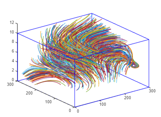
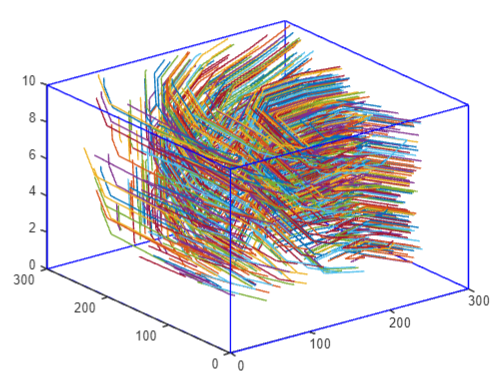
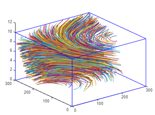
The following snippet plots the streamlines. First we plot the outline of the 3D domain and the last 3 code lines plot the actual streamlines
figure()
clf
plot3(domain_poly([1:4 1],1), domain_poly([1:4 1],2), 0*ones(1,5),'b')
hold on
plot3(domain_poly([1:4 1],1), domain_poly([1:4 1],2), 10*ones(1,5),'b')
for ii = 1:4
    plot3([domain_poly(ii,1);domain_poly(ii,1)], [domain_poly(ii,2);domain_poly(ii,2)], [0 10],'b')
end
for ii = 1:length(Snode)
plot3(Snode(ii,1).p(:,1), Snode(ii,1).p(:,2), Snode(ii,1).p(:,3))
end
By changing the Snode to Selem and Scloud we can print all of them as follows


Due to the very coarse discretization it is expected that the particle tracking resutls may be very different for each interpolation method even though the velocity fields are derived from the same data.
For the face interpolation we provide a separate example Simple Face Example on how to prepare the files.