PANOPLY Tutorial
PANOPLY is a platform for applying state-of-the-art statistical and machine learning algorithms to transform multi-omic data from cancer samples into biologically meaningful and interpretable results. PANOPLY leverages Terra—a cloud-native platform for extreme-scale data analysis, sharing, and collaboration—to host proteogenomic workflows, and is designed to be flexible, automated, reproducible, scalable, and secure. A wide array of algorithms applicable to all cancer types have been implemented, and we highlight the application of PANOPLY to the analysis of cancer proteogenomic data.
This PANOPLY tutorial provides a tour of how to use the PANOPLY proteogenomic data analysis pipeline, using the breast cancer dataset published in Mertins, et. al.1 The input dataset (tutorial-brca-input.zip file) can be found in the tutorial subdirectory, along with a HTML version of this tutorial.
- To run PANOPLY, you need a Terra account. To create an account follow the steps here. A Google account is required to create a Terra account.
- Once you have an account, you need to create a cloud billing account and project. Here, you will find step-by-step instructions to set up billing, including a free credits program for new users to try out Terra with $300 in Google Cloud credits.
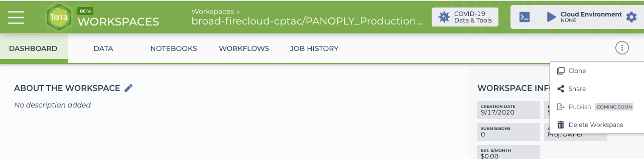
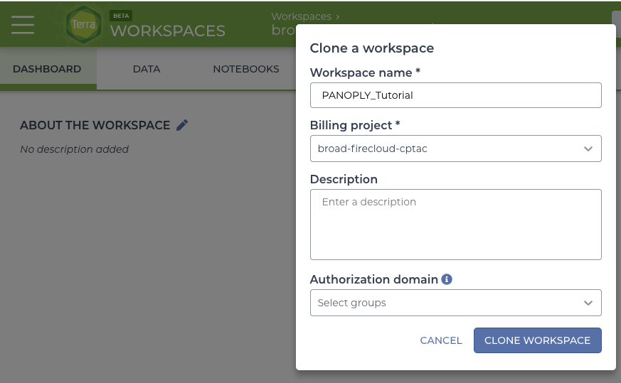
Clone the Terra production workspace at PANOPLY_Production_Pipelines_v1_4.
- Navigate to workspace. Click the circle with 3 dots at the top right and clone the workspace. When naming the new workspace, avoid special characters or spaces, and use only letters, numbers and underscores.
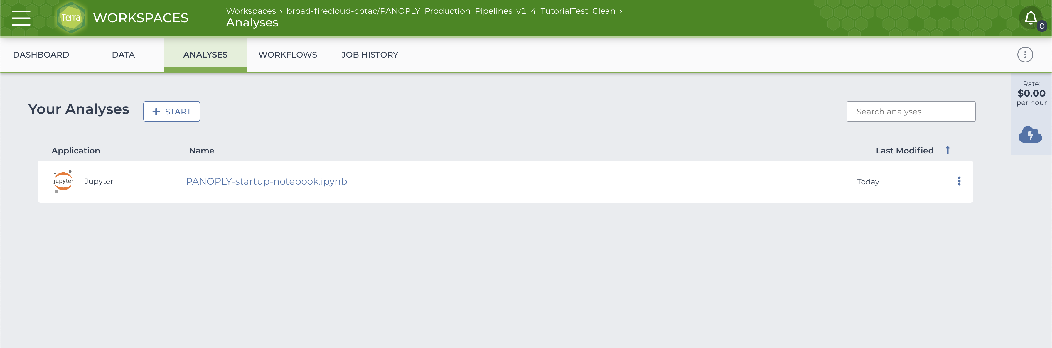
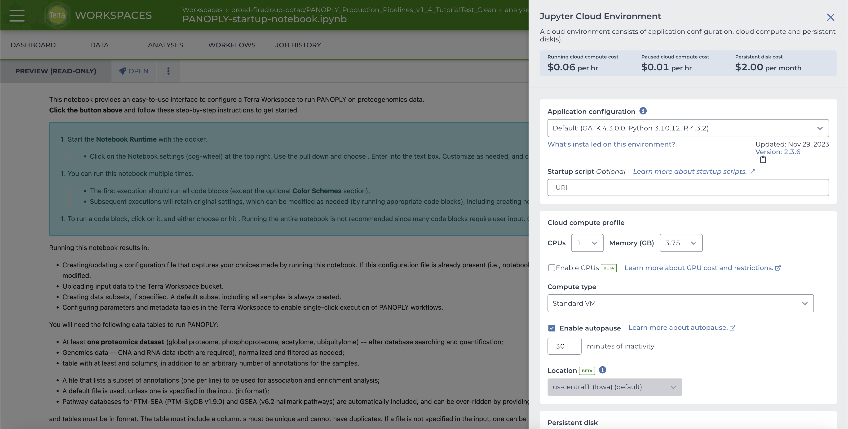
Select the NOTEBOOK tab and click on PANOPLY-startup-notebook.
The notebook is shown below:
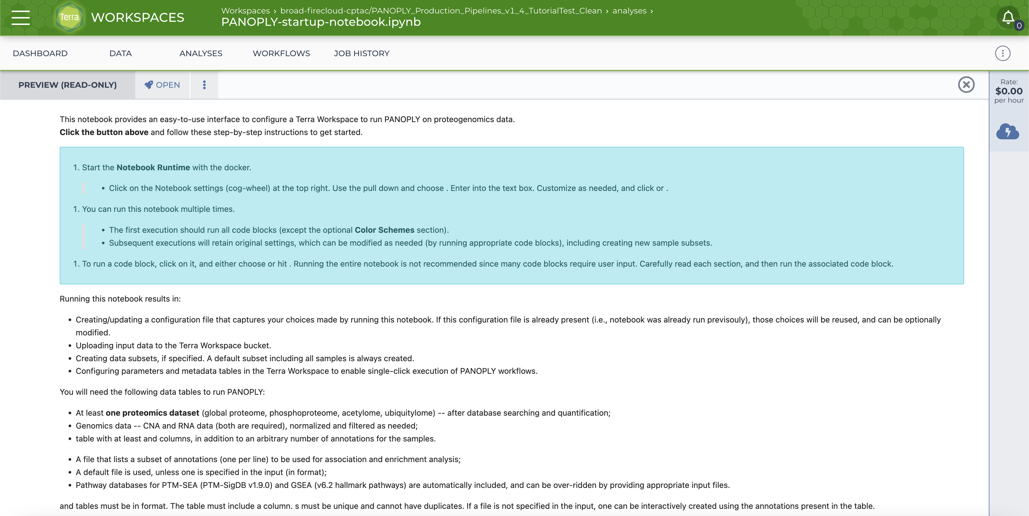
Click on the OPEN button on top. You will be prompted to start the Cloud Environment; the Cloud Environment popup will look like this:
To use the custom notebook docker, choose Custom Environment in the Application Configuration pull-down menu, and enter gcr.io/broadcptac/panda:1_4 in the Container image text box (A). Optionally, to improve runtime for larger datasets, increase CPUs to 4 and Memory to 15GB under Cloud Compute Profile (B).
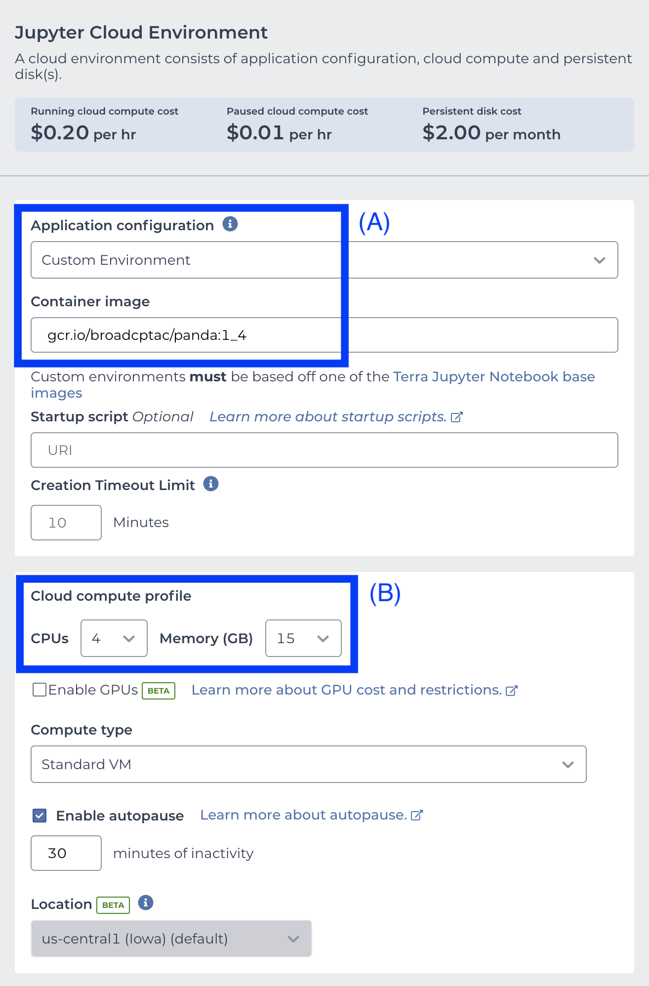
Then click NEXT at the bottom of the menu. Click CREATE when the Unverified Docker image page shows up. Once the Cloud Environment is running and the notebook is in EDIT mode (this may take a few minutes), read and follow the instructions in the notebook. In the notebook
-
Run the initialization code section by choosing
Cell -> Run Cellsor hittingShift-ENTER.:source( "/panda/build-config.r" ) panda_initialize("pipelines") -
The data has already been prepared and is available as a zip file here. Download this file to your local computer and then upload it to the google bucket using instructions in the
Upload ZIP file to workspace bucketsection of the notebook. Runpanda_datatypes()to list numerical mapping of allowable input data types. Then run
panda_input()provide the to uploaded input
zipfile as input and map files with datatypes as shown below:$$ Enter uploaded zip file name (test.zip): tutorial-brca-input.zip .. brca-retrospective-v5.0-cna-data.gct: 6 .. brca-retrospective-v5.0-phosphoproteome-ratio-norm-NArm.gct: 2 .. brca-retrospective-v5.0-proteome-ratio-norm-NArm.gct: 1 .. brca-retrospective-v5.0-rnaseq-data.gct: 5 .. brca-retrospective-v5.0-groups.csv: 8 .. brca-retrospective-v5.0-sample-annotation.csv: 7 .. msigdb_v7.0_h.all.v7.0.symbols.gmt: 11 ============================ .. INFO. Sample annotation file successfully validated. ============================ ============================ .. INFO. Validating sample IDs in all files. ============================ .. INFO. CNA successfully validated. .. INFO. PHOSPHOPROTEOME successfully validated. .. INFO. PROTEOME successfully validated. .. INFO. RNA successfully validated. ============================ .. INFO. Validating gene IDs in GCT files. ============================ .. INFO. Default Gene ID column 'geneSymbol' detected in CNA data. .. INFO. Default Gene ID column 'geneSymbol' detected in PHOSPHOPROTEOME data. .. INFO. Default Gene ID column 'geneSymbol' detected in PROTEOME data. .. INFO. Default Gene ID column 'geneSymbol' detected in RNA data. ============================ .. DONE. ============================ -
Run
panda_preprocessing()and toggle off proteome normalization, filtering, and PTM-SEA:
Does proteomics data need normalization? (y/n): n Does proteomics data need filtering? (y/n): n Phosphoproteome data detected. Should PTM-SEA be run? (y/n): n ============================ ============================ .. DONE. ============================ -
Provide
groups, or annotations of interest to be analyzed (e.g. enrichement analysis, outlier analysis, etc.). Agroupsfile is already included in the tutorial input to choose specific annotations for this purpose. Retain the groups file:max.categories <- 10 panda_groups()Groups file already present. Keep it? (y/n): y .. Selected groups: 1: PAM50 2: ER.Status 3: PR.Status 4: HER2.Status 5: TP53.mutation 6: PIK3CA.mutation 7: GATA3.mutation ============================ .. DONE. ============================ -
Skip down to the Sample Sets section and run
panda_sample_subsets()and do no add any additional sample subsets:
$$ Add additional sample subsets? (y/n): n
============================
.. Sample sets to be added to Terra Workspace:
.. all
============================
.. DONE.
============================
By default a sample set
allwill be created, containing all the input samples. -
Run
select_COSMO_attributes()and turn COSMO off:
Run COSMO? (y/n): n Select COSMO attributes anyways to run COSMO later? (y/n): n ============================ .. DONE. ============================ -
Finalize options:
panda_finalize()============================ .. DONE. ============================and run PANDA:
run_panda()This will take 5-10 minutes to read in all the input data types, populate the data model, and upload all the data to the google bucket associated with the workspace. After successful completion of
run_panda(), thesample_settable in theDATAtab will be populated, with the default sample-setallcontaining all samples,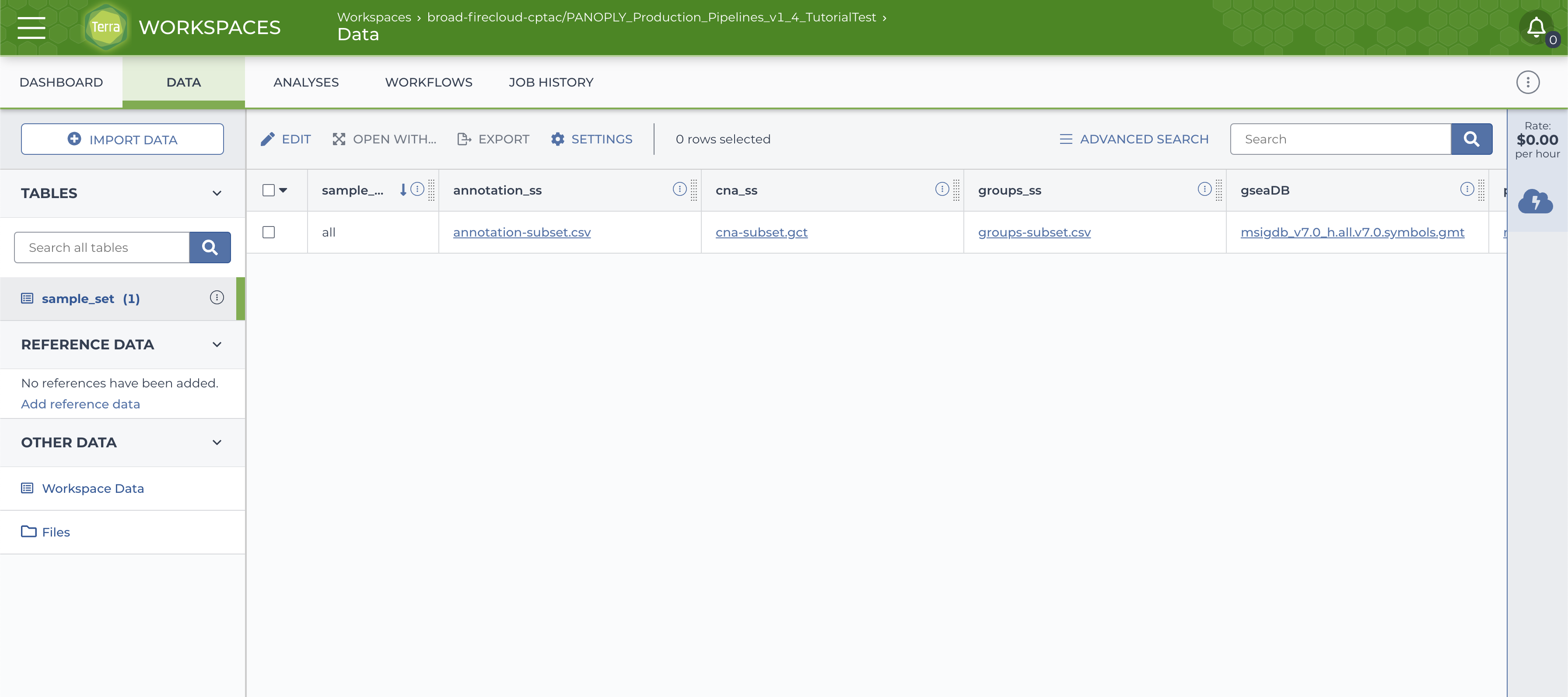
and a
sample_setdirectory with data files will be created on the google bucket (accessed via theFilesbutton on the left side in theDATAtab).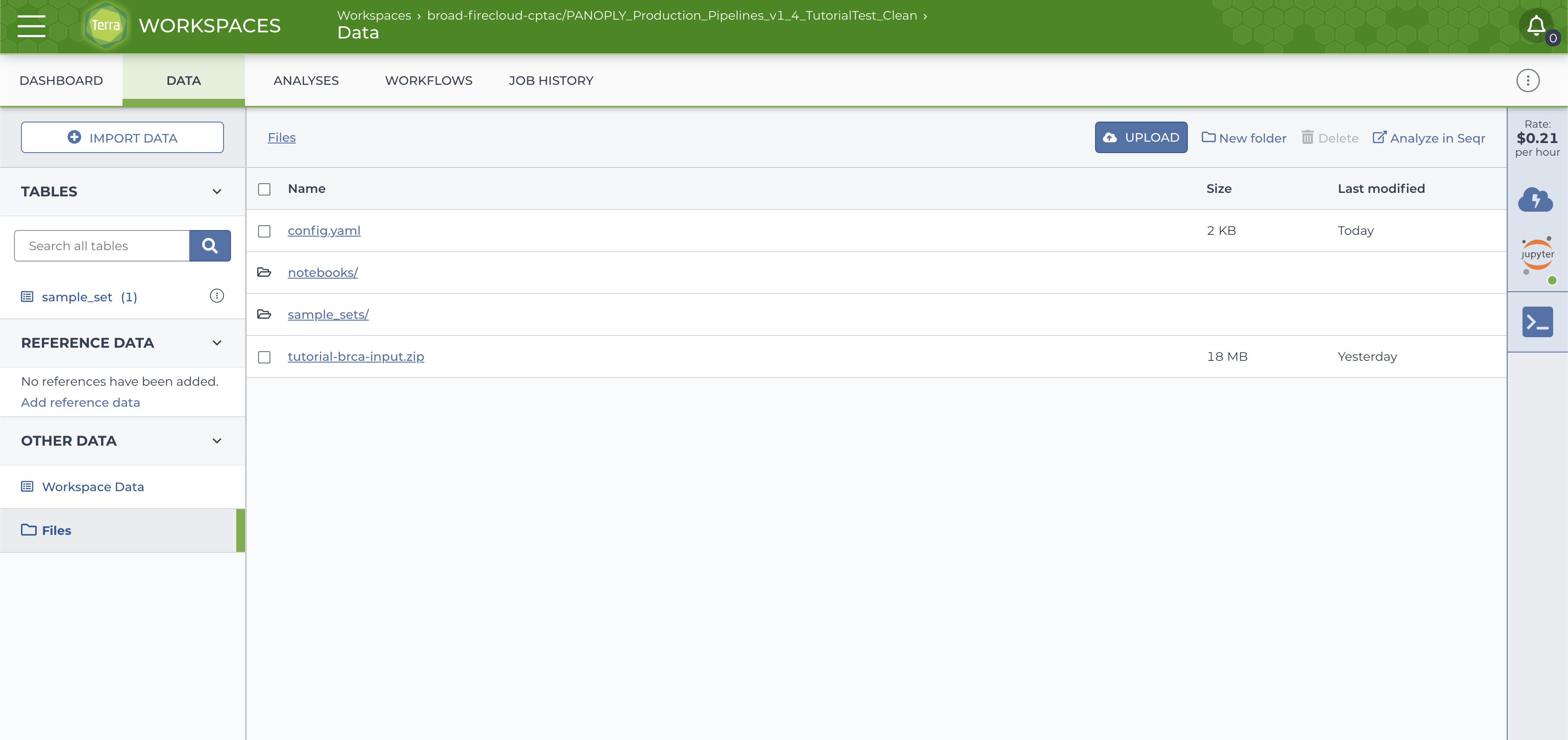
Once the startup notebook has completed running, and the data tables and files have been populated, navigate to the WORKFLOWS tab, locate the panoply_main_proteome workflow and click on it. A screen like the image below will appear:
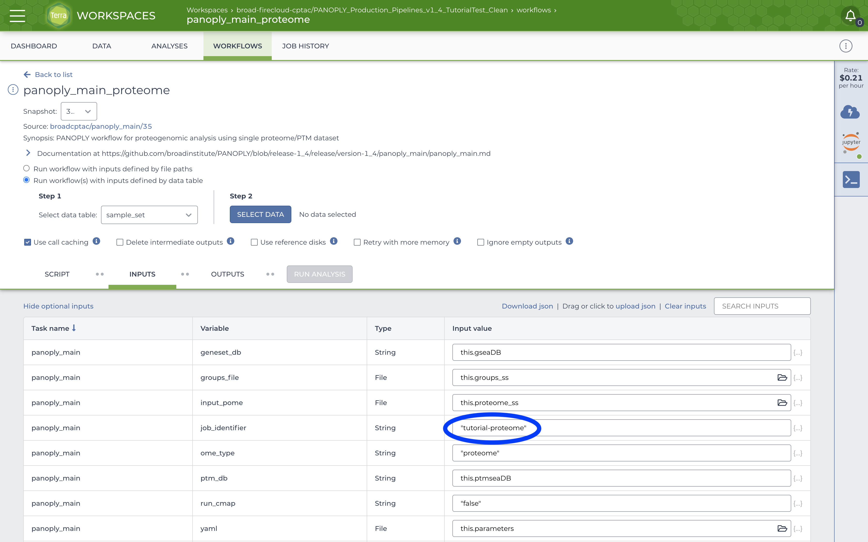
Fill out the job_identifier with an appropriate name. All other required (and some optional) inputs will be already correctly configured to use data tables created by running the startup notebook. Further, in the top section, ensure that:
- The
Run workflow(s) with inputs defined by data tableradio button is selected - Under
Step 1, the root entity type is set tosample_set
Click SELECT DATA under Step 2 and select the all sample_set:
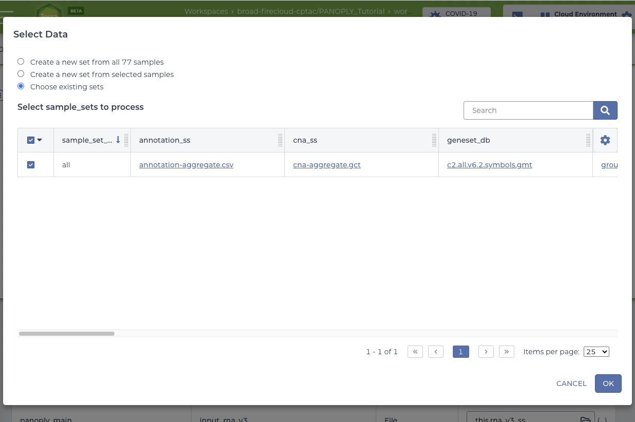
Click OK on the Select Data screen to return to the panoply_main_proteome workflow. Click SAVE to save your choices, at which point the RUN ANALYSIS button will be enabled. Note that all the required and optional input for the workflow are automatically filled in, and linked to appropriate data files in the Google bucket via columns in the data table.
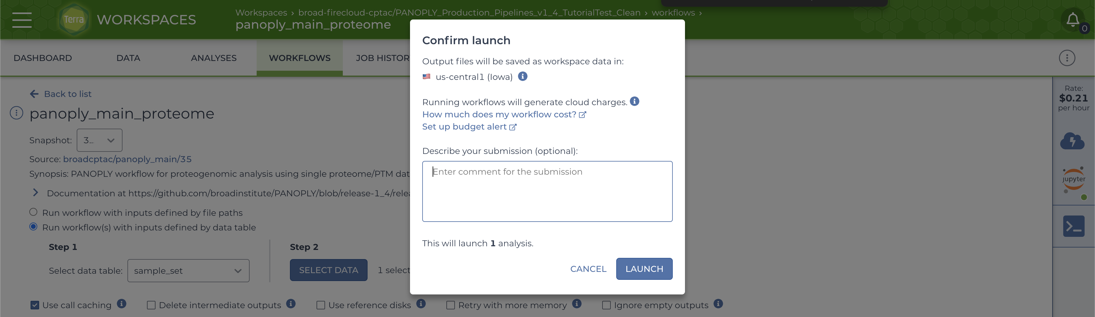
Start the workflow by clicking the RUN ANALYSIS button, and confirm launch by clicking the LAUNCH button on the popup:
The progress of the launched job can be monitored using the JOB HISTORY tab:
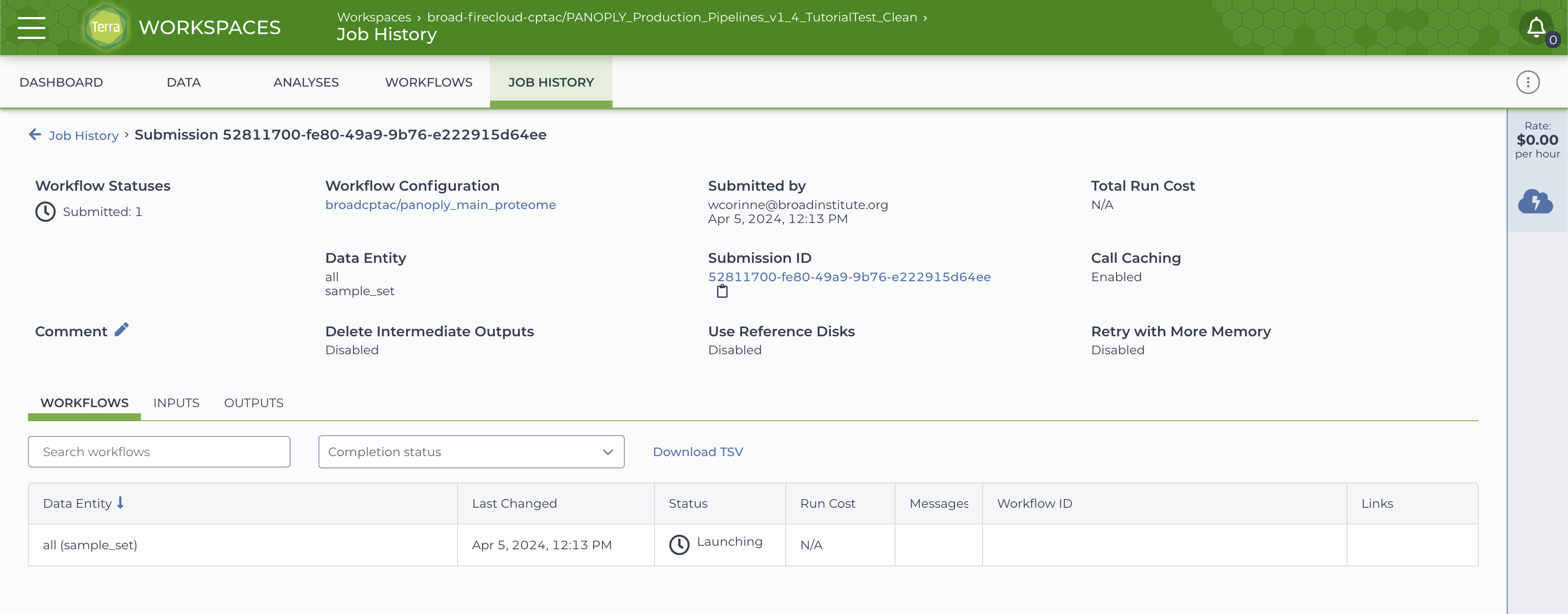
On successful completion of the submitted job, the JOB HISTORY tab will show a Succeeded status for the job.
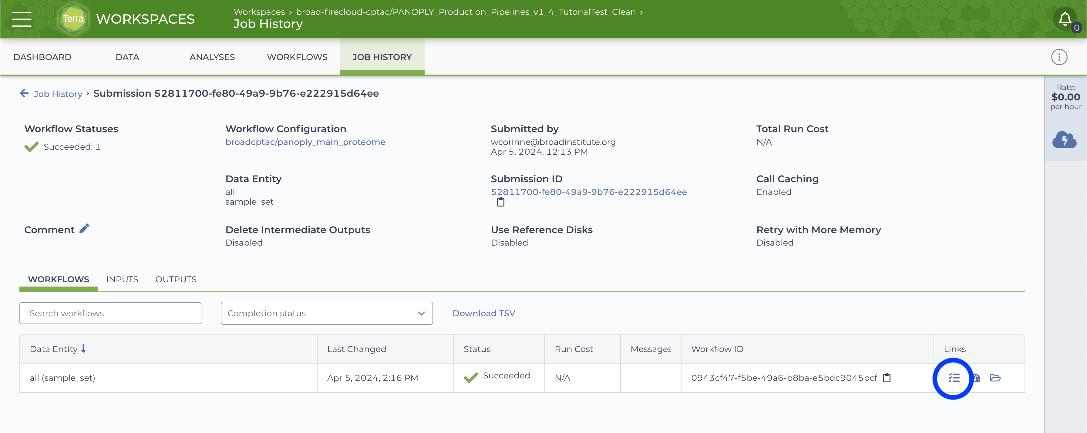
Click on the Job Manager icon (circled in blue in above) to get to the Job Manager page. Here, select the OUTPUTS tab to see all output files:
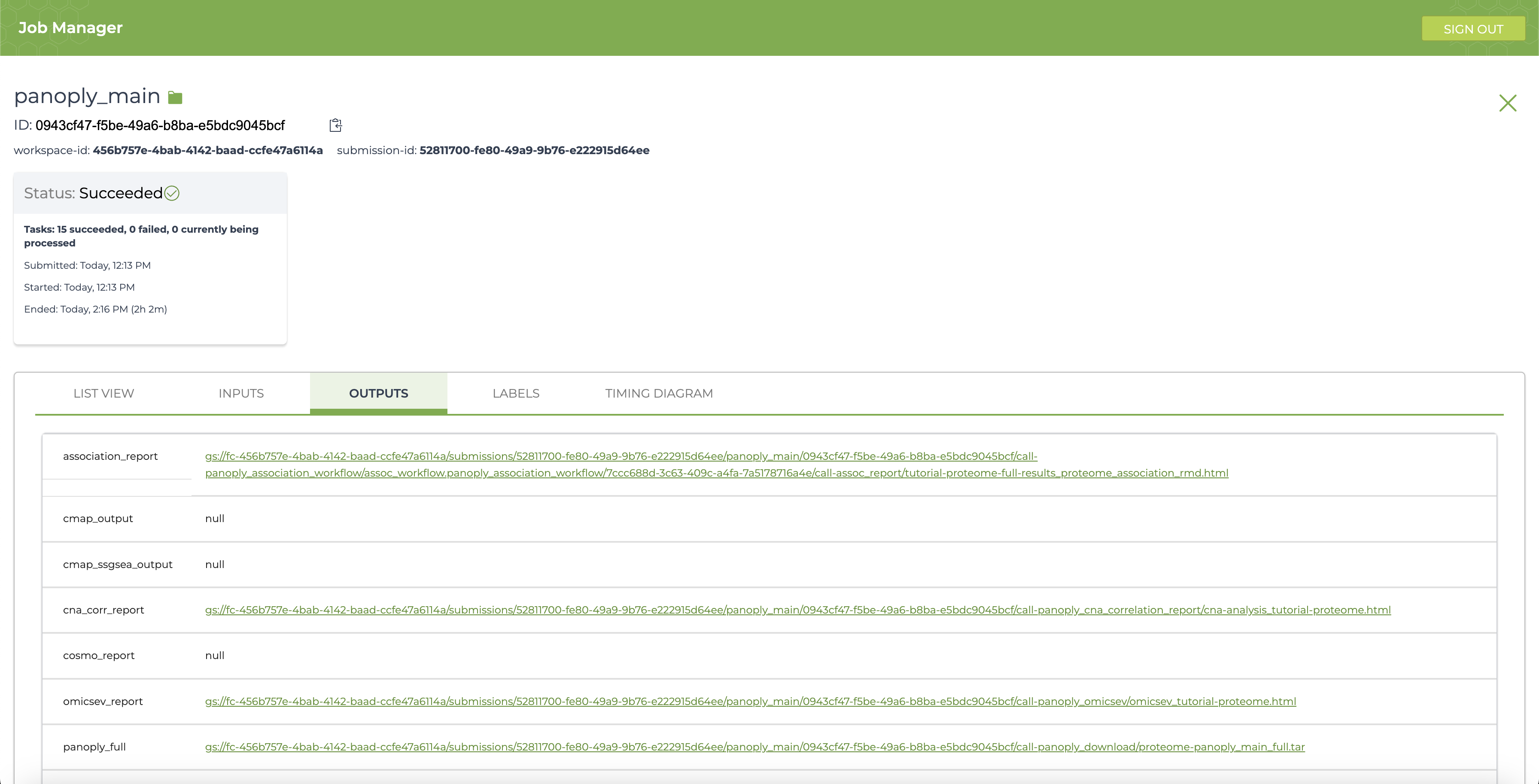
Running PANOPLY workflows generate several interactive *_reports that are HTML files with a summary of results from the appropriate analysis modules. In addition, all the reports with single-sample GSEA output is contained in the summary_and_ssgsea section. The complete output including all output tables, figures and results can be found in the file pointed to by panoply_full. All output files reside on the Google bucket associated with the execution workspace, and can be accessed by clicking on the links in the OUTPUTS page. Many files can be viewed directly by following the links, and all files can be downloaded either through the browser, or using the gsutil cp command in a terminal window. Detailed descriptions of the reports and results can be found at Navigating Results.
In a manner similar to running panoply_main_proteome (which runs the full proteogenomic analysis workflow for the global proteome data), the panoply_unified_workflow can also be run. This workflow automatically runs proteogenomic analysis for the proteome and phosphoproteome data, in addition to immune analysis (using panoply_immune_analysis), outlier analysis (using panoply_blacksheep) and NMF multi-omic clustering (using panoply_nmf). The panoply_unified_workflow can also run CMAP analysis (using panoply_cmap_analysis) but this modules is disabled, since running it can be expensive (about $150). The CMAP module can be enabled by setting run_cmap to "true". Again, all results and reports can be found under the OUTPUTS tab, with descriptions of reports at Navigating Results.
The table below summarizes expected time and cost for running various components of PANOPLY on the tutorial dataset. The table also provides ballpark estimates and ranges for each component assuming default parameter settings.
The time and cost can vary depending on runtime conditions, pre-emption of running jobs, and parameter settings. For example, increasing the number of random permutations for multi-omics NMF clusters (panoply_nmf) or CMAP analysis (panoply_cmap_analysis) will result in proportional increase in cost and time. Terra also includes a caching mechanism that reuses results for modules with no changes (to the module and input data/parameters). Enabling call caching can result in significant cost and time savings when only a few modules in a pipeline need to be rerun. In addition, Terra dispatches modules in parallel -- modules with input data available are run in parallel. This reduces total pipeline run time when compared to the cumulative time needed to run all modules.
| Item | Approx. Time (Range) | Approx. Cost (Range) | |
|---|---|---|---|
Startup Notebook to prepare workspace (panda) |
15 min (10-30 min) |
$1 ($0-$1) |
|
Main pipeline for proteome data (panoply_main) |
3.5 hr (3-4 hr) |
$2 ($1-$5) |
|
Unified pipeline for proteome+PTM, including NMF multi-omics clustering and CMAP analysis (panoply_unified_workflow) |
|||
| Total | 9.5 hr (8-10 hr) |
$55 ($50-$75) |
|
Main pipeline on proteome+PTM (panoply_main) |
4.5 hr (3-5 hr) |
$5 ($1-$10) |
|
Multi-omics NMF clustering (panoply_nmf) |
4 hr (3-4 hr) |
$25 ($15-$50) |
|
CMAP analysis (panoply_cmap_analysis) |
3 hr (2-3 hr) |
$25 ($15-$50) |
|
| Storage for input data + results of pipeline runs (~15 GB total) | $2-$3 / month |
- Mertins, P. et al. Proteogenomics connects somatic mutations to signalling in breast cancer. Nature 534, 55–62 (2016).